Quality control and manual segmentation

Overview

Questions

• What is segmentation?
• How do we manually segment images in Napari?

Objectives

• Explain some common quality control steps e.g. assessing an image’s histogram, checking clipping/dynamic range

• Explain what a segmentation, mask and label image are

• Create a label layer in Napari and use some of its manual segmentation tools (e.g. paintbrush/fill bucket)

For the next few episodes, we will work through an example of counting the number of cells in an image.

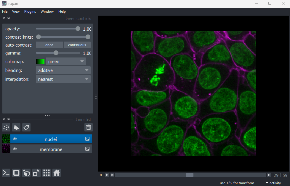
First, let’s open one of Napari’s sample images with:
File > Open Sample > napari builtins > Cells (3D + 2Ch)

Quality control

---

The first step in any image processing workflow is always quality control. We have to check that the images we acquired at the microscope capture the features we are interested in, with a reasonable signal to noise ratio (recall we discussed signal to noise ratio in the last episode).

In order to count our cells, we will need to see individual nuclei in our images. As there is one nucleus per cell, we will use the nucleus number as the equivalent of cell number. If we look at our cells image in Napari, we can clearly see multiple cell nuclei in green. If we zoom in we can see some noise (as a slight ‘graininess’ over the image), but this doesn’t interfere with being able to see the locations or sizes of all nuclei.

Next, it’s good practice to check the image histogram, as we covered in the choosing acquisition settings episode. We’ll do this in the exercise below:

Histogram quality control

Plot the image histogram with napari matplotlib:

• Do you see any issues with the histogram?

If you need a refresher on how to use napari matplotlib, check out the image display episode. It may also be useful to zoom into parts of the image histogram by clicking the icon at the top of histogram, then clicking and dragging a box around the region you want to zoom into. You can reset your histogram by clicking the icon.

Show me the solution

In the top menu bar of Napari select:
Plugins > napari Matplotlib > Histogram

Make sure you have the ‘nuclei’ layer selected in the layer list (should be highlighted in blue).

Z slices and contrast limits

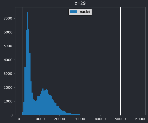
Note that as this image is 3D napari matplotlib only shows the histogram of the current z slice (in this case z=29 as shown at the top of the histogram). Moving the slider at the bottom of the viewer, will update the histogram to show different slices.

The vertical white lines at the left and right of the histogram display the current contrast limits as set in the layer controls. Note that by default Napari isn’t using the full image range as the contrast limits. We can change this by right clicking on the contrast limits slider and selecting the ‘reset’ button on the right hand side. This will set the contrast limits to the min/max pixel value of the current z slice. If we instead want to use the full 16-bit range from 0-65535, we can instead click the ‘full range’ button, then drag the contrast limit nodes to each end of the slider.

First, are there pixel values spread over most of the possible range? We can check what range is possible by printing the image’s data type to the console:

PYTHON

nuclei = viewer.layers["nuclei"].data
print(nuclei.dtype)

OUTPUT

uint16

This shows the image is an unsigned integer 16-bit image, which has a pixel value range from 0-65535 (as we covered in the ‘What is an image?’ episode). This matches the range on the x axis of our napari-matplotlib histogram.

If we look at the brightest part of the image, near z=29, we can see that there are indeed pixel values over much of this possible range. At first glance, it may seem like there are no values at the right side of the histogram, but if we zoom in using the icon we can clearly see pixels at these higher values.

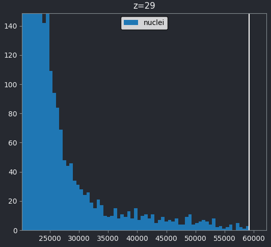
Most importantly, we see no evidence for ‘clipping’, which means we are avoiding any irretrievable loss of information this would cause. Recall that clipping occurs when pixels are recording light above the maximum limit for the image. Therefore, many values are ‘clipped’ to the maximum value resulting in information loss.

What is segmentation?

---

In order to count the number of cells, we must ‘segment’ the nuclei in this image. Segmentation is the process of labelling each pixel in an image e.g. is that pixel part of a nucleus or not? Segmentation comes in two main types - ‘semantic segmentation’ and ‘instance segmentation’. In this section we’ll describe what both kinds of segmentation represent, as well as how they relate to each other, using some simple examples.

First, let’s take a quick look at a rough semantic segmentation. Open Napari’s console by pressing the button, then copy and paste the code below. Don’t worry about the details of what’s happening in the code - we’ll look at some of these concepts like gaussian blur and otsu thresholding in later episodes!

PYTHON

from skimage.filters import threshold_otsu, gaussian

image = viewer.layers["nuclei"].data

blurred = gaussian(image, sigma=3)
threshold = threshold_otsu(blurred)

semantic_seg = blurred > threshold
viewer.add_labels(semantic_seg)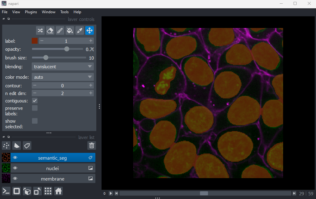

You should see an image appear that highlights the nuclei in brown. Try toggling the ‘semantic_seg’ layer on and off multiple times, by clicking the icon next to its name in the layer list. You should see that the brown areas match the nucleus boundaries reasonably well.

This is an example of a ‘semantic segmentation’. In a semantic segmentation, pixels are grouped into different categories (also known as ‘classes’). In this example, we have assigned each pixel to one of two classes: nuclei or background. Importantly, it doesn’t recognise which pixels belong to different objects of the same category - for example, here we don’t know which pixels belong to individual, separate nuclei. This is the role of ‘instance segmentation’ that we’ll look at next.

Copy and paste the code below into Napari’s console. Again, don’t worry about the details of what’s happening here - we’ll look at some of these concepts in later episodes.

PYTHON

from skimage.morphology import binary_erosion, ball
from skimage.segmentation import expand_labels
from skimage.measure import label

eroded = binary_erosion(semantic_seg, footprint=ball(10))
instance_seg = label(eroded)
instance_seg = expand_labels(instance_seg, distance=10)

viewer.add_labels(instance_seg)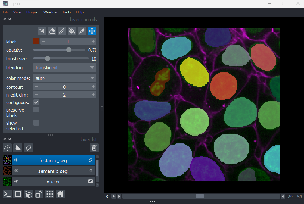

You should see an image appear that highlights nuclei in different colours. Let’s hide the ‘semantic_seg’ layer by clicking the icon next to its name in Napari’s layer list. Then try toggling the ‘instance_seg’ layer on and off multiple times, by clicking the corresponding icon. You should see that the coloured areas match most of the nucleus boundaries reasonably well, although there are some areas that are less well labelled.

This image is an example of an ‘instance segmentation’ - it is recognising which pixels belong to individual ‘instances’ of our category (nuclei). This is the kind of segmentation we will need in order to count the number of nuclei (and therefore the number of cells) in our image.

Note that it’s common for instance segmentations to be created by first making a semantic segmentation, then splitting it into individual instances. This isn’t always the case though - it will depend on the type of segmentation method you use.

How are segmentations represented?

---

How are segmentations represented in the computer? What pixel values do they use?

First, let’s focus on the ‘semantic_seg’ layer we created earlier:

• Click the icon next to ‘semantic_seg’ in the layer list to make it visible.
• Click the icon next to ‘instance_seg’ in the layer list to hide it.
• Make sure the ‘semantic_seg’ layer is selected in the layer list. It should be highlighted in blue.

Try hovering over the segmentation and examining the pixel values down in the bottom left corner of the viewer. Recall that we looked at pixel values in the ‘What is an image?’ episode.

You should see that a pixel value of 0 is used for the background and a pixel value of 1 is used for the nuclei. In fact, segmentations are stored in the computer in the same way as a standard image - as an array of pixel values. We can check this by printing the array into Napari’s console, as we did in the ‘What is an image?’ episode.

PYTHON

# Get the semantic segmentation data
image = viewer.layers['semantic_seg'].data

# Print the image values and type
print(image)
print(type(image))

Note the output is shortened here to save space!

OUTPUT

[[[0 0 0 ... 0 0 0]
  [0 0 0 ... 0 0 0]
  [0 0 0 ... 0 0 0]
  ...

<class 'numpy.ndarray'>

The difference between this and a standard image, is in what the pixel values represent. Here, they no longer represent the intensity of light at each pixel, but rather the assignment of each pixel to different categories or objects e.g.  0 = background, 1 = nuclei. You can also have many more values, depending on the categories/objects you are trying to represent. For example, we could have nucleus, cytoplasm, cell membrane and background, which would give four possible values of 0, 1, 2 and 3.

Let’s take a look at the pixel values in the instance segmentation:

• Click the icon next to ‘instance_seg’ in the layer list to make it visible.
• Click the icon next to ‘semantic_seg’ in the layer list to hide it.
• Make sure the ‘instance_seg’ layer is selected in the layer list. It should be highlighted in blue.

If you hover over the segmentation now, you should see that each nucleus has a different pixel value. We can find the maximum value via the console like so:

PYTHON

# Get the instance segmentation data
image = viewer.layers['instance_seg'].data

# Print the maximum pixel value
print(image.max())

OUTPUT

19

Instance segmentations tend to have many more pixel values, as there is one per object ‘instance’. When working with images with very large numbers of cells, you can quickly end up with hundreds or thousands of pixel values in an instance segmentation.

So to summarise - segmentations are just images where the pixel values represent specific categories, or individual instances of that category. You will sometimes see them referred to as ‘label images’, especially in the context of Napari. Segmentations with only two values (e.g. 0 and 1 for background vs some specific category) are often referred to as ‘masks’.

Note that in this episode we focus on segmentations where every pixel is assigned to a specific class or instance. There are many segmentation methods though that will instead output the probability of a pixel belonging to a specific class or instance. These may be stored as float images, where each pixel has a decimal value between 0 and 1 denoting their probability.

Segmentation shapes and data types

Copy and paste the following into Napari’s console:

PYTHON

nuclei = viewer.layers["nuclei"].data
semantic_seg = viewer.layers["semantic_seg"].data
instance_seg = viewer.layers["instance_seg"].data

• What shape are the nuclei, semantic_seg and instance_seg images?

• What pattern do you see in the shapes? Why?

• What bit-depth do the semantic_seg and instance_seg images have?

• If I want to make an instance segmentation of 100 nuclei - what’s the minimum bit depth I could use? (assume we’re storing unsigned integers) Choose from 8-bit, 16-bit or 32-bit.

• If I want to make an instance segmentation of 1000 nuclei - what’s the minimum bit depth I could use? (assume we’re storing unsigned integers) Choose from 8-bit, 16-bit or 32-bit.

Recall that we looked at image shapes and bit-depths in the ‘What is an image?’ episode.

Show me the solution

Shapes + pattern

PYTHON

print(nuclei.shape)
print(semantic_seg.shape)
print(instance_seg.shape)

OUTPUT

(60, 256, 256)
(60, 256, 256)
(60, 256, 256)

All the images have the same shape of (60, 256, 256). This makes sense as ‘semantic_seg’ and ‘instance_seg’ are segmentations made from the nuclei image. Therefore, they need to be exactly the same size as the nuclei image in order to assign a label to each pixel.

Note that even though the segmentation and image have the same shape, they often won’t have the same filesize when saved. This is due to segmentations containing many identical values (e.g. large parts of the image might be 0, for background) meaning they can often be compressed heavily without loss of information. Recall that we looked at compression in the filetypes and metadata episode.

Bit depths

PYTHON

print(semantic_seg.dtype)
print(instance_seg.dtype)

OUTPUT

int8
int32

The data type (.dtype) of ‘semantic_seg’ contains the number 8, showing that it is an 8-bit image. The data type of ‘instance_seg’ contains the number 32, showing that it is a 32-bit image.

Note that in this case, as the instance segmentation only contains 19 nuclei, it could also have been stored as 8-bit (and probably should have been, as this would provide a smaller file size!). The bit depth was increased by some of the image processing operations used to generate the instance segmentation, which is a common side effect as we’ll discuss in the next episode. If we wanted to reduce the bit depth, we could right click on the ‘instance_seg’ layer in the layer list, then select Convert data type. For more complex conversions, we would need to use python commands in Napari’s console - e.g. see the ‘Python: Types and bit-depths’ chapter form Pete Bankhead’s bioimage book.

Bit depth for 100 nuclei

To store an instance segmentation of 100 nuclei, we need to store values from 0-100 (with convention being that 0 represents the background pixels, and the rest are values for individual nuclei). An 8-bit unsigned integer image can store values from 0-255 and would therefore be sufficient in this case.

Bit depth for 1000 nuclei

To store an instance segmentation of 1000 nuclei, we need to store values from 0-1000 (with 0 being the background, and the rest values for individual nuclei). A 16-bit unsigned integer image can store values from 0-65535 and would therefore be sufficient in this case.

How to create segmentations?

---

There are many, many different methods for creating segmentations! These range from fully manual methods where you ‘paint’ the pixels in each category, to complicated automated methods relying on classical machine learning or deep learning models. The best method to use will depend on your research question and the type of images you have in your datasets. As we’ve mentioned before, it’s usually best to use the simplest method that works well for your data. In this episode we’ll look at manual methods for segmentation within Napari, before moving on to more automated methods in later episodes.

Manual segmentation in Napari

---

Let’s look at how we can create our own segmentations in Napari. First remove the two segmentation layers:

• Click on ‘instance_seg’, then shift + click ‘semantic_seg’
• Click the icon to remove these layers.

Then click on the icon (at the top of the layer list) to create a new Labels layer.

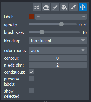
Recall from the imaging software episode, that Napari supports different kinds of layers. For example, Image layers for standard images, Point layers for points, Shape layers for shapes like rectangles, ellipses or lines etc… Labels layers are the type used for segmentations, and provide access to many new settings in the layer controls:

Let’s start by painting an individual nucleus. Select the paintbrush by clicking the icon in the top row of the layer controls. Then click and drag across the image to label pixels. You can change the size of the brush using the ‘brush size’ slider in the layer controls. To return to normal movement, you can click the icon in the top row of the layer controls, or hold down spacebar to activate it temporarily (this is useful if you want to pan slightly while painting). To remove painted areas, you can activate the label eraser by clicking the icon.

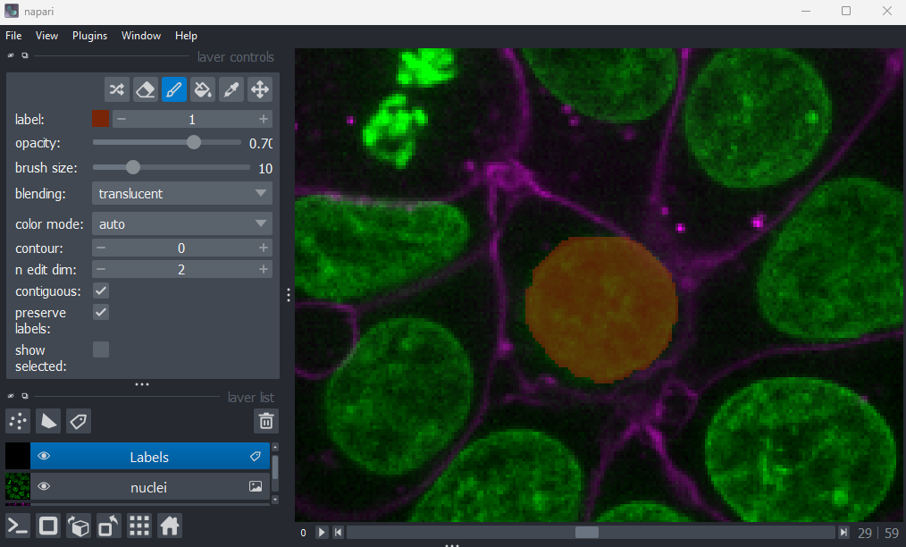
If you hover over the image and examine the pixel values, you will see that all your painted areas have a pixel value of 1. This corresponds to the number shown next to ‘label:’ in the layer controls.

To paint with a different pixel value, either click the + icon on the right side of this number, or type another value into the box. Let’s paint another nucleus with a pixel value of 2:

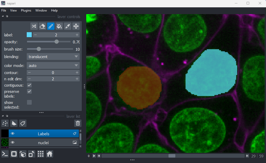
When you paint with a new value, you’ll see that Napari automatically assigns it a new colour. This is because Labels layers use a special colormap/LUT for their pixel values. Recall from the image display episode that colormaps are a way to convert pixel values into corresponding colours for display. The colormap for Labels layers will assign random colours to each pixel value, trying to ensure that nearby values (like 2 vs 3) are given dissimilar colours. This helps to make it easier to distinguish different labels. You can shuffle the colours used by clicking the icon in the top row of the layer controls. Note that the pixel value of 0 will always be shown as transparent - this is because it is usually used to represent the background.

Manual segmentation in Napari

Try labelling more individual nuclei in this image, making sure each gets its own pixel value (label). Investigate the other settings in the layer controls:

• What does the icon do?
• What does the icon do?
• What does the ‘contour’ setting control?
• What does the ‘n edit dim’ setting control?
• What does the ‘preserve labels’ setting control?

Remember that you can hover over buttons to see a helpful popup with some more information. You can also look in Napari’s documentation on Labels layers.

Note that if you make a mistake you can use Ctrl + Z to undo your last action. If you need to re-do it use Shift + Ctrl + Z.

Show me the solution

icon

This icon activates the ‘fill bucket’. It will fill whatever label you click on with the currently active label (as shown next to ‘label:’ in the layer controls). For example, if your active label is 2, then clicking on a nucleus with label 1 will change it to 2. You can see more details about the fill bucket in Napari’s documentation

icon

This icon activates the ‘colour picker’. This allows you to click on a pixel in the viewer and immediately select the corresponding label. This is especially useful when you have hundreds of labels, which can make them difficult to keep track of with the ‘label:’ option only.

Contour

The contour setting controls how labels are displayed. By default (when 0), labelled pixels are displayed as solid colours. Increasing the contour value to one or higher, will change this to show the outline of labelled regions instead. Higher values will result in a thicker outline. This can be useful if you don’t want to obscure the underlying image while viewing your segmentation.

n edit dim

This controls the number of dimensions that are used for editing labels. By default, this is 2 so all painting and editing of the Labels layer will only occur in 2D. If you want to paint/edit in 3D you can increase this to 3. Now painting will not only affect the currently visible image slice, but slices above and below it also. Be careful with the size of your brush when using this option!

preserve labels

Activating ‘preserve labels’ will ensure that any painting/erasing you do will only affect your currently active label. This is especially useful if you need to paint very close to existing labels without affecting them.

Manual vs automated?

---

Now that we’ve done some manual segmentation in Napari, you can probably tell that this is a very slow and time consuming process (especially if you want to segment in full 3D!). It’s also difficult to keep the segmentation fully consistent, especially if multiple people are contributing to it. For example, it can be difficult to tell exactly where the boundary of a nucleus should be placed, as there may be a gradual fall off in pixel intensity at the edge rather than a sharp drop.

Due to these challenges, full manual segmentation is generally only suitable for small images in small quantities. If we want to efficiently scale to larger images in large quantities, then we need more automated methods. We’ll look at some of these in the next few episodes, where we investigate some ‘classic’ image processing methods that generate segmentations directly from image pixel values. These automated approaches will also help us achieve a less variable segmentation, that segments objects in a fully consistent way.

For more complex segmentation scenarios, where the boundaries between objects are less clear, we may need to use machine learning or deep learning models. These models learn to segment images based on provided ‘groundtruth’ data. This ‘groundtruth’ is usually many small, manually segmented patches of our images of interest. While generating this manual groundtruth is still slow and time consuming, the advantage is that we only need to segment a small subset of our images (rather than the entire thing). Also, once the model is trained, it can be re-used on similar image data.

It’s worth bearing in mind that automated methods are rarely perfect (whether they’re classic image processing, machine learning or deep learning based). It’s very likely that you will have to do some manual segmentation cleanup from time to time.

Key Points

• The first step in any image processing workflow is quality control. For example, checking the histograms of your images.

• Segmentation is the process of identifying what each pixel in an image represents e.g. is that pixel part of a nucleus or not?

• Segmentation can be broadly split into ‘semantic segmentation’ and ‘instance segmentation’. Semantic segmentation assigns pixels to specific classes (like nuclei or background), while instance segmentation assigns pixels to individual ‘instances’ of a class (like individual nuclei).

• Segmentations are represented in the computer in the same way as standard images. The difference is that pixel values represent classes or instances, rather than light intensity.

• Napari uses Labels layers for segmentations. These offer various annotation tools like the paintbrush, fill bucket etc.

• Fully manual segmentation is generally only suitable for small images. More automated approaches (based on classic image processing, machine learning or deep learning) are necessary to scale to larger images. Even with automated methods, manual segmentation is often still a key component - both for generating groundtruth data and cleaning up problematic areas of the final segmentation.