Multi-dimensional images

Overview

Questions

• How do we visualise and work with images with more than 2 dimensions?

Objectives

• Explain how different axes (xyz, channels, time) are stored in image arrays and displayed
• Open and navigate images with different dimensions in Napari
• Explain what RGB images are and how they are handled in Napari
• Split and merge channels in Napari

Image dimensions / axes

---

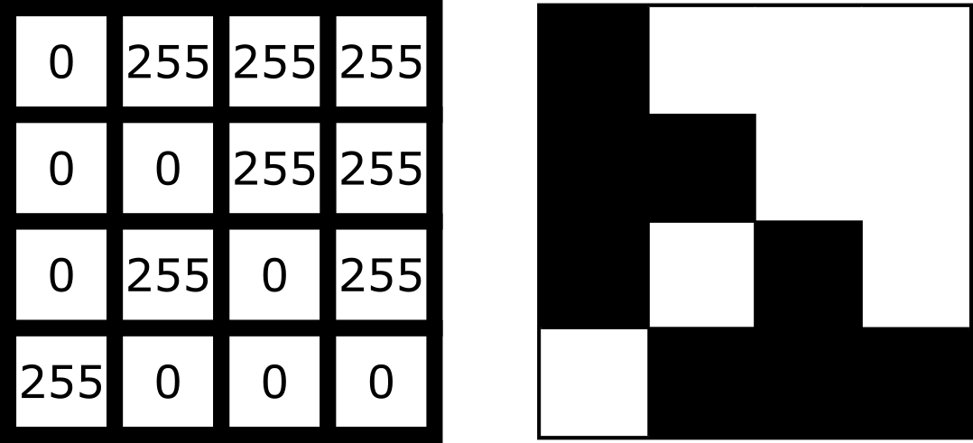
As we saw in the ‘What is an image?’ episode, image pixel values are stored as arrays of numbers with certain dimensions and data type. So far we have focused on grayscale 2D images that are represented by a 2D array:

Light microscopy data varies greatly though, and often has more dimensions representing:

• Time (t):
  Multiple images of the same sample over a certain time period - also known as a ‘time series’. This is useful to evaluate dynamic processes.

• Channels (c):
  Usually, this is multiple images of the same sample under different wavelengths of light (e.g. red, green, blue channels, or wavelengths specific to certain fluorescent markers). Note that channels can represent many more values though, as we will see below.

• Depth (z):
  Multiple images of the same sample, taken at different depths. This will produce a 3D volume of images, allowing the shape and position of objects to be understood in full 3D.

These images will be stored as arrays that have more than two dimensions. Let’s start with our familiar human mitosis image, and work up to some more complex imaging data.

2D

---

Go to the top menu-bar of Napari and select:
File > Open Sample > napari builtins > Human Mitosis

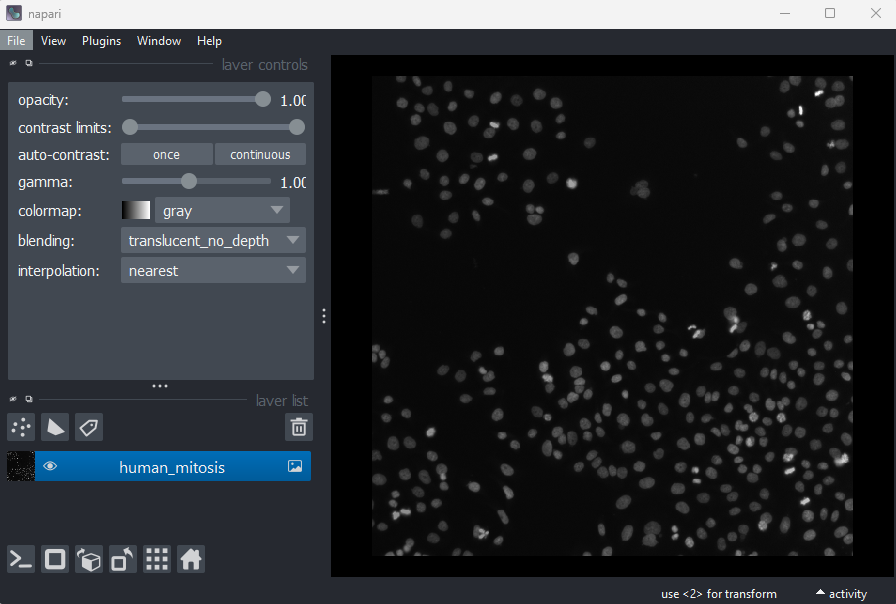
We can see this image only has two dimensions (or two ‘axes’ as they’re also known) due to the lack of sliders under the image, and by checking its shape in the Napari console. Remember that we looked at how to open the console and how to check the .shape in detail in the ‘What is an image?’ episode:

PYTHON

image = viewer.layers["human_mitosis"].data
print(image.shape)

OUTPUT

# (y, x)
(512, 512)

Note that comments have been added to all output sections in this episode (the lines starting with #). These state what the dimensions represent (e.g. (y, x) for the y and x axes). These comments won’t appear in the output in your console.

3D

---

Let’s remove the mitosis image by clicking the remove layer button at the top right of the layer list. Then, let’s open a new 3D image:
File > Open Sample > napari builtins > Brain (3D)

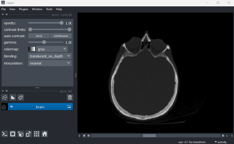
This image shows part of a human head acquired using X-ray Computerised Tomography (CT). We can see it has three dimensions due to the slider at the base of the image, and the shape output:

PYTHON

image = viewer.layers["brain"].data
print(image.shape)

OUTPUT

# (z, y, x)
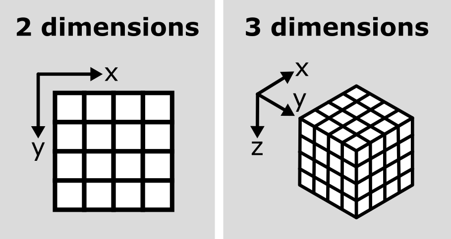
(10, 256, 256)

This 3D image can be thought of as a stack of ten 2D images, with each image containing a 256x256 array. The x/y axes point along the width/height of the first 2D image, and the z axis points along the stack. It is stored as a 3D array:

In Napari (and Python in general), dimensions are referred to by their index e.g. here dimension 0 is the z axis, dimension 1 is the y axis and dimension 2 is the x axis. We can check this in Napari by looking at the number at the very left of the slider. Here it’s labelled ‘0’, showing that it controls movement along dimension 0 (i.e. the z axis).

Axis labels

By default, sliders will be labelled by the index of the dimension they move along e.g. 0, 1, 2… Note that it is possible to re-name these though! For example, if you click on the number at the left of the slider, you can freely type in a new value. This can be useful to label sliders with informative names like ‘z’, or ‘time’.

You can also check which labels are currently being used with:

PYTHON

viewer.dims.axis_labels

Channels

---

Next, let’s look at a 3D image where an additional (fourth) dimension contains data from different ‘channels’. Remove the brain image and select:
File > Open Sample > napari builtins > Cells (3D+2Ch)

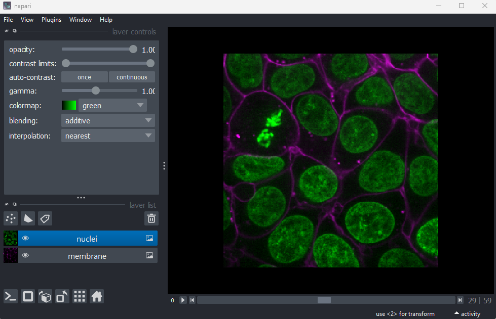
Image channels can be used to store data from multiple sources for the same location. For example, consider the diagram below. On the left is shown a 2D image array overlaid on a simple cell with a nucleus. Each of the pixel locations e.g. (0, 0), (1, 1), (2, 1)… can be considered as sampling locations where different measurements can be made. For example, this could be the intensity of light detected with different wavelengths (like red, green…) at each location, or it could be measurements of properties like the surface height and elasticity at each location (like from scanning probe microscopy). These separate data sources are stored as ‘channels’ in our image.

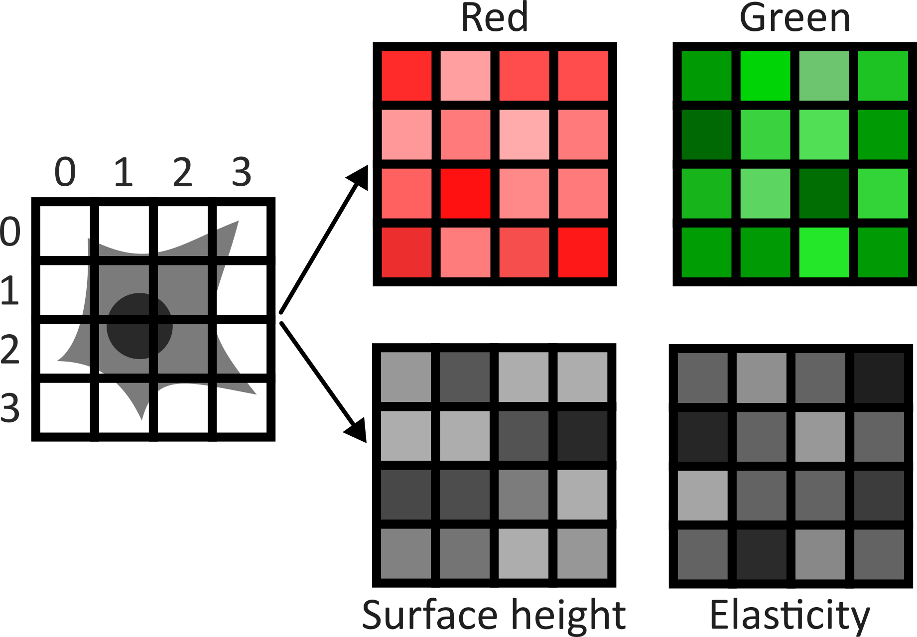
This diagram shows an example of a 2D image with channels, but this can also be extended to 3D images, as we will see now.

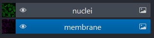
Fluorescence microscopy images, like the one we currently have open in Napari, are common examples of images with multiple channels. In flourescence microscopy, different ‘flourophores’ are used that target specific features (like the nucleus or cell membrane) and emit light of different wavelengths. Images are taken filtering for each of these wavelengths in turn, giving one image channel per fluorophore. In this case, there are two channels - one for a flourophore targeting the nucleus, and one for a fluorophore targeting the cell membrane. These are shown as separate image layers in Napari’s layer list:

Recall from the imaging software episode that ‘layers’ are how Napari displays multiple items together in the viewer. Each layer could be an entire image, part of an image like a single channel, a series of points or shapes etc. Each layer is displayed as a named item in the layer list, and can have various display settings adjusted in the layer controls.

Let’s check the shape of both layers:

PYTHON

nuclei = viewer.layers["nuclei"].data
membrane = viewer.layers["membrane"].data
print(nuclei.shape)
print(membrane.shape)

OUTPUT

# (z, y, x)
(60, 256, 256)
(60, 256, 256)

This shows that each layer contains a 3D image array of size 60x256x256. Each 3D image represents the intensity of light detected at each (z, y, x) location with a wavelength corresponding to the given fluorophore.

Here, Napari has automatically recognised that this image contains different channels and separated them into different image layers. This is not always the case though, and sometimes it may be preferable to not split the channels into separate layers! We can merge our channels again by selecting both image layers (shift + click so they’re both highlighted in blue), right clicking on them and selecting:
Merge to stack

You should see the two image layers disappear, and a new combined layer appear in the layer list (labelled ‘membrane’). This image has an extra slider that allows switching channels - try moving both sliders and see how the image display changes.

We can check the image’s dimensions with:

PYTHON

image = viewer.layers["membrane"].data
print(image.shape)

OUTPUT

# (c, z, y, x)
(2, 60, 256, 256)

Notice how these dimensions match combining the two layers shown above. Two arrays with 3 dimensions (60, 256, 256) are combined to give one array with four dimensions (2, 60, 256, 256) with the first axis representing the 2 channels. See the diagram below for a visualisation of how these 3D and 4D arrays compare:

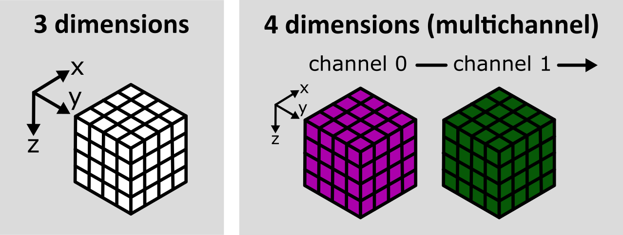
As we’ve seen before, the labels on the left hand side of each slider in Napari matches the index of the dimension it moves along. The top slider (labelled 1) moves along the z axis, while the bottom slider (labelled 0) switches channels.

We can separate the channels again by right clicking on the ‘membrane’ image layer and selecting:
Split Stack

Note that this resets the contrast limits for membrane and nuclei to defaults of the min/max possible values. You’ll need to adjust the contrast limits on the membrane layer to see it clearly again after splitting.

Reading channels in Napari

When we open the cells image through the Napari menu, it is really calling something like:

from skimage import data
viewer.add_image(data.cells3d(), channel_axis=1)

This adds the cells 3D image (which is stored as zcyx), and specifies that dimension 1 is the channel axis. This allows Napari to split the channels automatically into different layers.

Usually when loading your own images into Napari e.g. with the napari-aicsimageio plugin (as we will see in the filetypes and metadata episode), the channel axis should be recognised automatically. If not, you may need to add the image via the console as above, manually stating the channel axis.

When to split channels into layers in Napari?

As we saw above, we have two choices when loading images with multiple channels into Napari:

• Load the image as one Napari layer, and use a slider to change channel

• Load each channel as a separate Napari layer, e.g. using the channel_axis

Both are useful ways to view multichannel images, and which you choose will depend on your image and preference. Some pros and cons are shown below:

Pros and cons

Channels as separate layers

1. Channels can be overlaid on top of each other (rather than only viewed one at a time)

2. Channels can be easily shown/hidden with the icons

3. Display settings like contrast limits and colormaps can be controlled independently for each channel (rather than only for the entire image)

Entire image as one layer

1. Useful when handling a very large number of channels. For example, if we have hundreds of channels, then moving between them on a slider may be simpler and faster.

2. Napari can become slow, or even crash with a very large number of layers. Keeping the entire image as one layer can help prevent this.

3. Keeping the full image as one layer can be helpful when running certain processing operations across multiple channels at once

Time

---

You should have already downloaded the MitoCheck dataset as part of the setup instructions - if not, you can download it by clicking on ‘00001_01.ome.tiff’ on this page of the OME website.

To open it in Napari, remove any existing image layers, then drag and drop the file over the canvas. A popup may appear asking you to choose a ‘reader’ - you can select either ‘napari builtins’ or ‘napari-aicsimageio’. We’ll see in the next episode that the ‘napari-aicsimageio’ reader gives us access to useful image metadata.

Note this image can take a while to open, so give it some time! Alternatively, you can select in the top menu-bar:
File > Open File(s)...

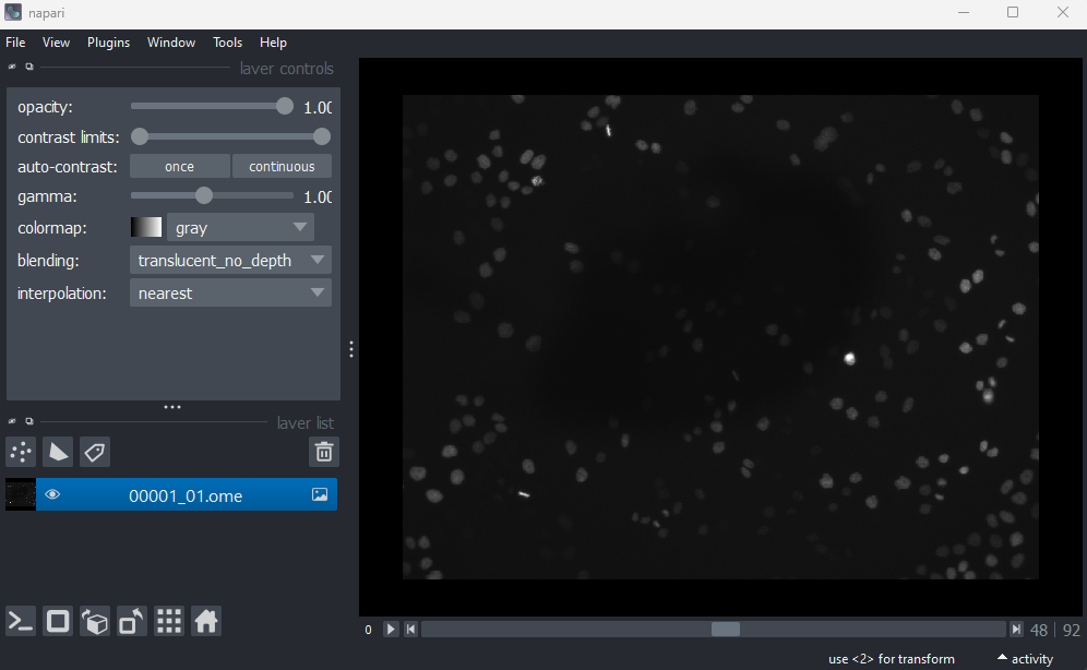
This image is a 2D time series (tyx) of some human cells undergoing mitosis. The slider at the bottom now moves through time, rather than z or channels. Try moving the slider from left to right - you should see some nuclei divide and the total number of nuclei increase. You can also press the small icon at the left side of the slider to automatically move along it. The icon will change into a - pressing this will stop the movement.

We can again check the image dimensions by running the following:

PYTHON

image = viewer.layers["00001_01.ome"].data
print(image.shape)

OUTPUT

# (t, y, x)
(93, 1024, 1344)

Note that this image has a total of 3 dimensions, and so it will also be stored in a 3D array:

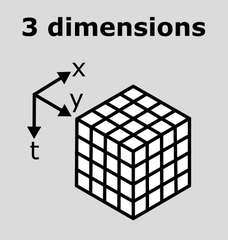
This makes the point that the dimensions don’t always represent the same quantities. For example, a 3D image array with shape (512, 512, 512) could represent a zyx, cyx or tyx image. We’ll discuss this more in the next section.

Dimension order

---

As we’ve seen so far, we can check the number and size of an image’s dimensions by running:

PYTHON

image.shape

Napari reads this array and displays the image appropriately, with the correct number of sliders, based on these dimensions. It’s worth noting though that Napari doesn’t usually know what these different dimensions represent e.g.  consider a 4 dimensional image with shape (512, 512, 512, 512). This could be tcyx, czyx, tzyx etc… Napari will just display it as an image with 2 additional sliders, not caring about exactly what each represents.

Python has certain conventions for the order of image axes (like scikit-image’s ‘coordinate conventions’ and aicsimageio’s reader) - but this tends to vary based on the library or plugin you’re using. These are not firm rules!

Therefore, it’s always worth checking you understand which axes are being shown in any viewer and what they represent! Check against your prior knowledge of the experimental setup, and check the metadata in the original image (we’ll look at this in the next episode). If you want to change how axes are displayed, remember you can use the roll or transpose dimensions buttons as discussed in the imaging software episode. Also, if loading the image manually from the console, you can provide some extra information like the channel_axis parameter discussed above.

Interpreting image dimensions

Remove all image layers, then open a new image by copying and pasting the following into Napari’s console:

PYTHON

from skimage import data
image = viewer.add_image(data.kidney(), rgb=False).data

This is a fluorescence microscopy image of mouse kidney tissue.

1. How many dimensions does it have?

2. What do each of those dimensions represent? (e.g. t, c, z, y, x) Hint: try using the roll dimensions button to view different combinations of axes.

3. Once you know which dimension represent channels, remove the image and load it again with:

PYTHON

# Replace ? with the correct channel axis
viewer.add_image(data.kidney(), rgb=False, channel_axis=?)

Note that using the wrong channel axis may cause Napari to crash. If this happens to you just restart Napari and try again. Bear in mind, as we saw in the channel splitting section that large numbers of layers can be difficult to handle, so it isn’t usually advisable to use ‘channel_axis’ on dimensions with a large size.

4. How many channels does the image have?

Show me the solution

1

The image has 4 dimensions, which we can see with:

PYTHON

image.shape

OUTPUT

(16, 512, 512, 3)

2

If we press the roll dimensions button once, we can see an image of various cells and nuclei. Moving the slider labelled ‘0’ seems to move up and down in this image (i.e. the z axis), while moving the slider labelled ‘3’ changes between highlighting different features like nuclei and cell edges (i.e. channels). Therefore, the remaining two axes (1 and 2) must be y and x. This means the image’s 4 dimensions are (z, y, x, c)

3

The channel axis is 3 (remember that the numbering always starts form 0!)

4

There are 3 channels which we can see from the .shape output, or from the number of layers in the layer list.

RGB

---

For the final part of this episode, let’s look at RGB images. RGB images can be considered as a special case of a 2D image with channels (yxc). In this case, there are always 3 channels - with one representing red (R), one representing green (G) and one representing blue (B).

Let’s open an example RGB image with the command below. Make sure you remove any existing image layers first!
File > Open Sample > napari builtins > Skin (RGB)

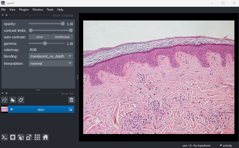
This image is a hematoxylin and eosin stained slide of dermis and epidermis (skin layers). Let’s check its shape:

PYTHON

image = viewer.layers["skin"].data
print(image.shape)

OUTPUT

# (y, x, c)
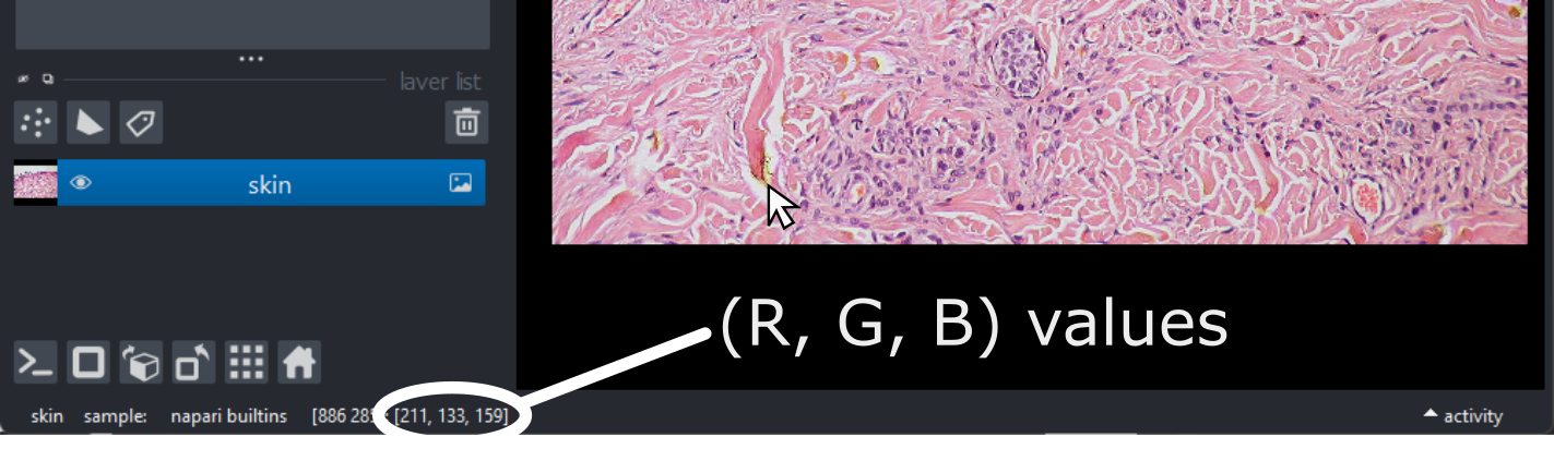
(960, 1280, 3)

Notice that the channels aren’t separated out into different image layers, as they were for the multichannel images above. Instead, they are shown combined together as a single image. If you hover your mouse over the image, you should see three pixel values printed in the bottom left representing (R, G, B).

We can see these different channels more clearly if we right click on the ‘skin’ image layer and select:
Split RGB

This shows the red, green and blue channels as separate image layers. Try inspecting each one individually by clicking the icons to hide the other layers.

We can understand these RGB pixel values better by opening a different sample image. Remove all layers, then select:
File > Open Sample > napari builtins > Colorwheel (RGB)

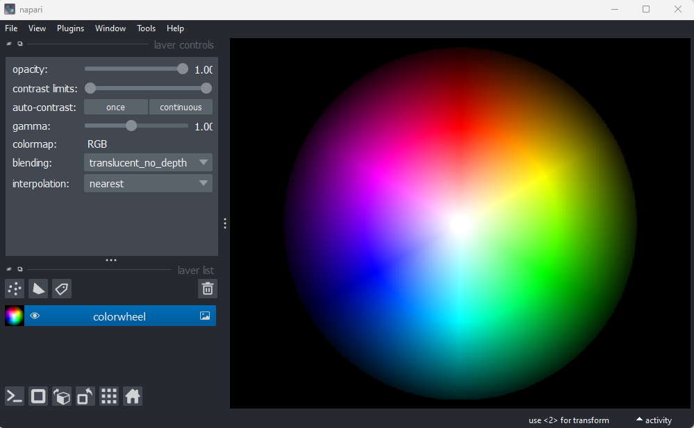
This image shows an RGB colourwheel - try hovering your mouse over different areas, making note of the (R, G, B) values shown in the bottom left of Napari. You should see that moving into the red area gives high values for R, and low values for B and G. Equally, the green area shows high values for G, and the blue area shows high values for B. The red, green and blue values are mixed together to give the final colour.

Recall from the image display episode that for most microscopy images the colour of each pixel is determined by a colormap (or LUT). Each pixel usually has a single value that is then mapped to a corresponding colour via the colormap, and different colormaps can be used to highlight different features. RGB images are different - here we have three values (R, G, B) that unambiguously correspond to a colour for display. For example, (255, 0, 0) would always be fully red, (0, 255, 0) would always be fully green and so on… This is why there is no option to select a colormap in the layer controls when an RGB image is displayed. In effect, the colormap is hard-coded into the image, with a full colour stored for every pixel location.

These kinds of images are common when we are trying to replicate what can be seen with the human eye. For example, photos taken with a standard camera or phone will be RGB. They are less common in microscopy, although there are certain research fields and types of microscope that commonly use RGB. A key example is imaging of tissue sections for histology or pathology. You will also often use RGB images when preparing figures for papers and presentations - RGB images can be opened in all imaging software (not just scientific research focused ones), so are useful when preparing images for display. As usual, always make sure you keep a copy of your original raw data!

Reading RGB in Napari

How does Napari know an image is RGB? If an image’s final dimension has a length of 3 or 4, Napari will assume it is RGB and display it as such. If loading an image from the console, you can also manually set it to load as rgb:

PYTHON

from skimage import data
viewer.add_image(data.astronaut(), rgb=True)

RGB histograms

Make a histogram of the Skin (RGB) image using napari-matplotlib (as covered in the image display episode)

• How does it differ from the image histograms we looked at in the image display episode?

Show me the solution

If you haven’t completed the image display episode, you will need to install the napari-matplotlib plugin.

Then open a histogram with:
Plugins > napari Matplotlib > Histogram

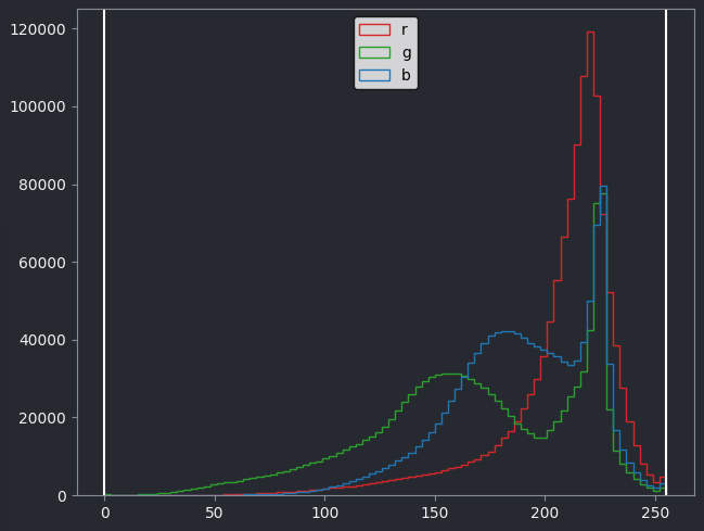
This histogram shows separate lines for R, G and B - this is because each displayed pixel is represented by three values (R, G, B). This differs from the histograms we looked at previously, where there was only one line as each displayed pixel was only represented by one value.

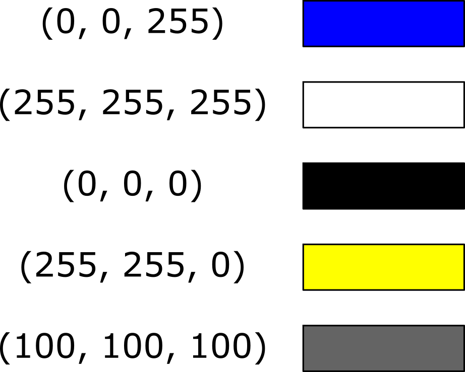
Understanding RGB colours

What colour would you expect the following (R, G, B) values to produce? Each value has a minimum of 0 and a maximum of 255.

• (0, 0, 255)
• (255, 255, 255)
• (0, 0, 0)
• (255, 255, 0)
• (100, 100, 100)

Show me the solution

Key Points

• Microscopy images can have many dimensions, usually representing time (t), channels (c), and spatial axes (z, y, x)
• Napari can open images with any number of dimensions
• Napari (and python in general) has no firm rules for axis order. Different libraries and plugins will often use different conventions.
• RGB images always have 3 channels - red (R), green (G) and blue (B). These channels aren’t separated into different image layers - they’re instead combined together to give the final image display.