Choosing acquisition settings
Last updated on 2026-06-09 | Edit this page
Overview
Questions
- What are the key factors to consider when choosing acquisition settings?
Objectives
Explain some examples of acquisition settings, and factors to consider when choosing them
Explain the difference between resolution and pixel size
Describe some quality control steps e.g. monitoring the image histogram
In the last episode we looked at some of the main steps to designing a light microscopy experiment:
Define your research question
Define what you need to observe to answer that question
Define what you need to measure to answer that question
Choose a light microscopy method that fits your data needs
Choose acquisition settings that fit your data needs
In this episode, we’ll focus on the last step - choosing acquisition settings - as well as looking at some early quality control steps.
Acquisition settings
Once you’ve chosen a light microscope to use, there are a wide variety of acquisition settings that can be adjusted. Acquisition settings commonly optimised for an experiment include magnification, laser power, and exposure time, but there are many others. Different combinations of settings will be best for different samples and research questions. For example, one combination of settings may be best for rapid live cell imaging, while another may be best for high resolution imaging of fixed samples.
There are many different factors that are affected by acquisition settings, but here are some of the main ones to consider.
Spatial resolution
Spatial resolution is defined as the smallest distance between two adjacent points on a sample that can still be seen as separate entities. In 2D, this is measured in x and y, while in 3D it is measured in x, y and z. For example, a resolution of one micrometre would mean that objects less than one micrometre apart couldn’t be identified separately (i.e. they would appear as one object).
Spatial resolution is affected by many factors including the wavelength of light and the numerical aperture (NA) of the objective lens. Using a shorter wavelength of light and higher NA lenses, can provide higher resolution images.
Spatial resolution can be isotropic (the same in all directions) or anisotropic (different in different directions). Anisotropic resolution is common with 3D datasets, where the x/y resolution tends to be better than the z resolution.
We’ll look at spatial resolution in more detail later in this episode.
Spatial resolution and optical resolution
In this episode, we use ‘spatial resolution’ to refer to the resolution limits of the light microscope. Note that sometimes ‘spatial resolution’ is also used to refer to the final image pixel size (as we will look at later in this episode). Due to this ambiguity, you may also see the microscope’s resolution referred to as ‘optical resolution’ to clearly distinguish it from pixel size.
Temporal resolution
Temporal (or time) resolution, is how fast images can be acquired (usually measured in seconds or milliseconds). This is mainly controlled by the ‘exposure time’, which is the length of time over which the detector collects light for each image. For a laser scanning confocal microscope, you will instead see a ‘dwell time’ - this is the time the laser spends illuminating each position on the sample. Decreasing exposure time / dwell time will result in faster overall imaging speeds.
The imaging speed will also depend on some of the mechanical properties of your chosen light microscope. For example, the speed with which a laser-scanning confocal can move the laser across a sample, or (if imaging multiple locations) the speed of the microscope stage movement.
To produce good quality images (with a high signal-to-noise ratio, as we’ll look at later), the detector needs to collect as much light as possible in these short timescales.
Field of view
The field of view is the size of the area you can view with your light microscope. It is often measured as a diameter in millimetres. A larger field of view is useful if you want to, for example, observe a large number of cells at the same time. This can quickly increase your sample size, providing improved statistical power (as covered in the last episode).
The field of view is affected by many factors but, importantly, is directly related to the magnification of the objective lens. Higher levels of magnification result in a smaller field of view.
To image areas larger than the field of view, you will need to acquire multiple images at different positions by moving the microscope’s stage. These images can then be stitched together (often with the microscope manufacturer’s acquisition software), to give one large final image. This method can provide high resolution images of large areas, but also slows down overall acquisition times.
Depth penetration
Depth penetration refers to the distance light can penetrate into your sample (in the z direction). It therefore controls the maximum z range that you can image over - for example, a specific confocal microscope may be limited to a maximum depth of 50 micrometre.
Depth penetration is limited due to samples absorbing and scattering light that passes through them. Various factors control the penetration depth - for example, the density of the sample and the wavelength of light used during imaging. Various tissue clearing methods exist that can help to make a sample more transparent, and allow imaging at greater depths. Also, the use of longer wavelengths of light can reduce absorption/scattering and increase depth penetration. This comes at the cost of decreased spatial resolution (as we covered in the spatial resolution section). For very thick samples, you will likely need to use a microscope specialised for this task e.g. a multiphoton microscope.
Data size
It’s important to consider the overall size of your imaging data (e.g. in megabytes (MB), gigabytes (GB) or terabytes (TB)). Light microscopy datasets can be extremely large in size, so you will have to make sure you have appropriate file storage space that is regularly backed up.
The overall size of your data will depend on many factors. For example, increasing your resolution will increase the size of your final images, especially if you are covering a large area by stitching multiple images taken at different positions together.
Light exposure (i.e phototoxicity / photobleaching)
Illuminating our samples with light is an essential part of collecting light microscopy images. However, we must also be mindful of the detrimental effects light can have on our samples, especially at high intensity over long time periods.
Photobleaching is a key issue for fluorescence microscopy. If a fluorophore is exposed to intense light, its structure can degrade over time. This means that it will eventually stop fluorescing entirely.
Another issue is phototoxicity. Light exposure can damage cells resulting in unexpected changes in cell behaviour, morphology and eventually cell death.
Reducing the effects of photobleaching and phototoxicity requires minimising the light exposure of our samples as much as possible. Light exposure can be reduced through many methods, including reducing light/laser power, reducing exposure time/dwell time, and imaging at lower temporal resolution.
Signal to noise ratio
Signal to noise ratio is a very useful measure of image quality - in general, it will be easier to identify and measure features of interest in images with a higher signal to noise ratio.
The ‘signal’ is what we really want to measure - for example, for a fluorescence microscopy image, this would be the light emitted by fluorophores in the sample. In an ideal world the detector would perfectly measure the light intensity, but this isn’t really possible. The values the detector records will always be affected by random fluctuations called ‘noise’ (see the ‘where does noise come from?’ section for more information). This noise usually appears as a random ‘graininess’ over the image and can make details difficult to see.
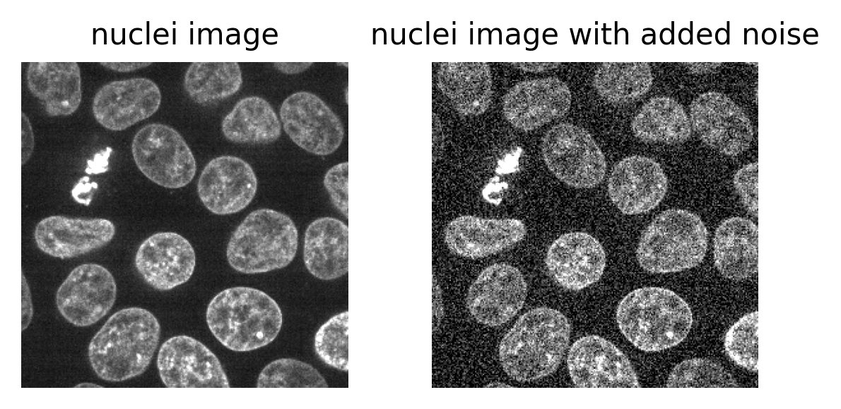
To identify and measure our features of interest, the absolute size of the signal and noise are less important than the ratio between them. For example, imagine we are trying to distinguish between two areas with different brightness - one being 1.5x brighter than the other. In a low signal setup where values are small (say 20 vs 30) adding noise can make these areas very difficult to separate. For example, see the diagram below which shows three histograms. The left is the ideal scenario, where there is no noise, and we perfectly see one value of 20 and one of 30. The middle shows the addition of some noise to each value, resulting in wider distributions that overlap extensively. This means that in the combined histogram of these values (right) it becomes impossible to clearly distinguish these two values. Note - here the added noise is a gaussian distribution centred on each value (i.e. 20 and 30) with a standard deviation of 10 and 1000 samples - you can read more about gaussian noise in the noise chapter of Pete Bankhead’s bioimage book.
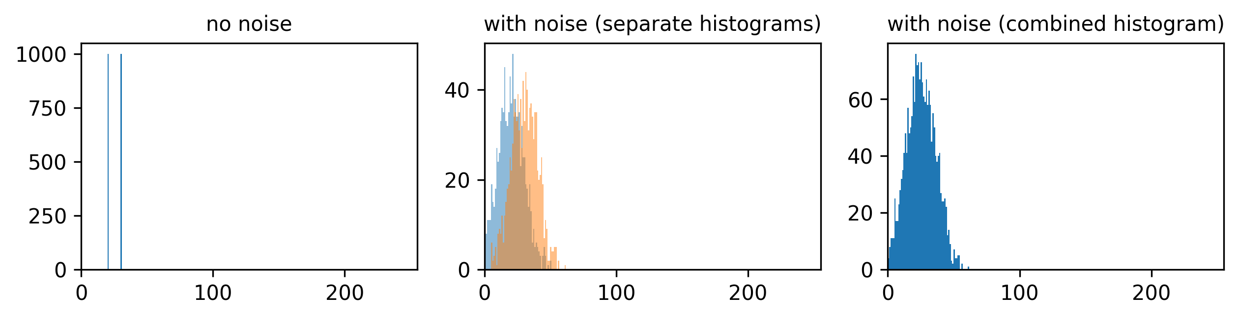
If we imagine a scenario with higher signal, now values of 80 and 120 (one still 1.5x higher than the other), then we can see that adding the same level of noise has less effect. As the values are now higher and further apart, the broadening of their distributions only causes them to overlap slightly. We can still clearly distinguish the values in the combined histogram on the right. This demonstrates how increasing the signal to noise ratio can improve our ability to recognise and measure different features.
How can we improve the signal to noise ratio of our images? The main solution is to increase the amount of light that we detect per image, by adjusting our acquisition settings. For example:
- increase light/laser power
- increase exposure time / dwell time
- Use binning (this combines multiple pixels into a single larger pixel)
- Average multiple images
If you want to find out more about noise, we recommend the noise chapter of Pete Bankhead’s bioimage book.
Where does noise come from?
Noise comes from many sources - for example, ‘photon noise’ (also known as ‘shot noise’) is a key source. Photon noise is caused by inherent statistical fluctuations in the emission of photons (individual light ‘packets’). For example, consider a fluorescence microscopy experiment where photons of light are being emitted from a fluorescent label. Even though the average rate of emission is constant, the exact number of photons emitted in a specific time interval (say 30 seconds) will vary each time. Say 20 photons, then 18, then 22… The exact time a photon is emitted is random, so there will always be random variations. These follow a statistical distribution known as a ‘poisson distribution’ - if you’re interested in the details Pete Bankhead’s bioimage book has a great chapter on noise.
The important point to consider is that there will always be some photon noise. It is inherit noise in the emission of light, and therefore not dependent on a particular microscope or detector setup.
Other types of noise are dependent on the microscope itself, often associated with the kind of detector used. For example, ‘read noise’ and ‘dark noise’ are commonly associated with CCD (charge-coupled device) cameras. These types of noise relate to slight inaccuracies in quantifying the number of photons that hit the detector - no detector is perfect, so there will always be some variation.
Optimising acquisition settings
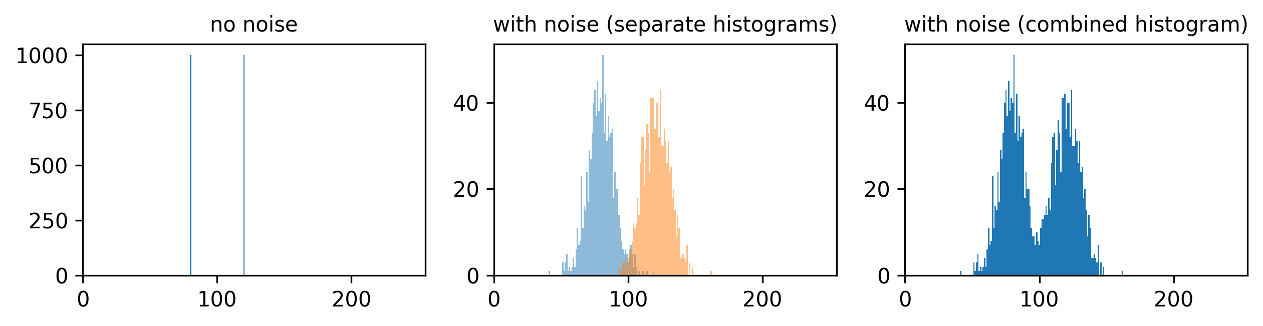
In an ideal world we could produce the ‘perfect’ image that optimised for all of the features above: high spatial resolution, high temporal resolution, large field of view, large depth penetration, small data size, low light exposure and high signal to noise ratio. This is never possible though! There are always trade-offs and compromises to be made. These different factors are inter-related, usually meaning that optimising for one will be at the expense of the others. For example, increasing spatial resolution requires a reduced field of view, and it will increase the overall data size. As each pixel covers a smaller area, resulting in less signal per pixel, you will likely need to increase light exposure to achieve a comparable signal to noise ratio. This may mean using higher light intensity, or imaging more slowly (with increased dwell time/exposure time).
Different microscopes will provide different ranges for these features - for example, supporting different ranges of spatial or temporal resolution, or providing detectors with different sensitivity that require higher or lower light intensity. Acquisition settings then allow you to fine-tune how that microscope functions, optimising within these ranges for your particular sample and research question. For example, do you need to prioritise temporal resolution for a highly dynamic process? Or perhaps is spatial resolution the priority, as your region of interest is very small?
Jonkman et al.’s 2020 paper provides some great advice for choosing confocal microscopes and acquisition settings, with figure 5 as a great example of the different trade-offs.
Choosing acquisition settings
In the previous episode, we used an example of investigating the effects of a specific chemical on cells grown in culture. Continuing with this, which acquisition settings would we need to prioritise to answer our research question? - ‘Does the chemical affect the number, size or shape of cell nuclei over time?’
Think about the points above and the trade-offs between them to make a list of potential answers. It may be best to discuss in a group, so you can share different ideas.
There’s no one correct answer here, as it will depend on which type of light microscope you are using and which aspects of nucleus size and shape you want to focus on. Here are some points to consider though:
Light exposure
As we are interested in how the nuclei number, shape and size changes over time, we will need to use live cell imaging. Light exposure (photobleaching / phototoxicity) can be a huge issue for these long experiments where cells must be exposed to light again and again. Therefore, to image for as long as possible, we should try to reduce light exposure as much as possible. This may require using lower resolution, lower light/laser power and shorter exposure times. We must balance this against signal to noise ratio though.
Data size and spatial resolution
As we are taking many images over a long timescale, our data size could become very large. To minimise this, we should make sure we are using the lowest spatial resolution possible (that still lets us see individual nucleus size/shape). Usually this means selecting a lower NA objective lens (which is usually also a lower magnification objective lens).
Also, we should ensure we are using an appropriate interval between our images. For example, do you need an image every minute? Or is every ten minutes fine? Longer intervals will reduce the size of your final dataset.
Temporal resolution
If we are only interested in measuring overall changes in the mean nucleus number / size / shape, we can afford to have quite large intervals between our images (low temporal resolution). If we instead wanted to track the progress of individual nuclei over time (e.g. their movements and individual divisions), we would need much smaller intervals (higher temporal resolution).
Field of view
We will need to keep the field of view large enough to image many nuclei at once - this will give us a good estimate of the average nuclei number / shape / size. This means we should use the lowest magnification objective lens that still provides enough spatial resolution to see individual nuclei. Alternatively, we will need to stitch images together from multiple positions - although this will slow down acquisition, and must be balanced against the required temporal resolution!
Depth penetration
As we are considering cells grown in culture (rather than in thick tissues), depth penetration isn’t a key concern here. This means we shouldn’t have to, for example, limit ourselves to fluorophores with longer emission wavelengths, or require any additional preparation steps like tissue clearing.
Resolution vs pixel size
Let’s dive deeper into choosing an appropriate spatial resolution for your experiment. First, let’s clarify the differences between magnification, pixel size and spatial resolution.
Spatial resolution
As defined above, spatial resolution is the smallest distance between two points on a sample that can still be seen as separate entities. It is a measure of the microscope’s ability to resolve small details in an image.
Magnification
Magnification describes how much larger an object appears through the microscope vs its actual size e.g. 10x larger, 100x larger…
\[ \large \text{Magnification} = \frac{\text{Size of object in microscopy image}}{\text{True size of object}} \]
Note that this is not the same as spatial resolution! Magnification just describes how large an object appears, not the size of the details it can resolve. For example, a particular light microscope may have a maximum spatial resolution of one micrometre - meaning that it won’t be able to discern features less than this distance apart. It may be possible to magnify images far beyond this limit though, making them appear larger and larger without allowing us to see any more detail. This is known as ‘empty magnification’ and should be avoided.
Pixel size
We discussed pixel size in the filetypes and metadata episode, but let’s recap here. The pixel size states how large a single image pixel is in physical units i.e. ‘real world’ units of measurement like micrometre, or millimetre.
Note again that this is not the same as the spatial resolution! The pixel size helps us understand how large a region each pixel of our image covers, but (as with magnification) it doesn’t tell us the size of details the microscope is really capable of resolving. For example, I could process a microscopy image to artificially give it 4x as many pixels as the original. This would reduce the pixel size without allowing us to see any smaller details i.e. there’s no corresponding improvement in spatial resolution!
Pixel size vs resolution
Consider the 16x16 pixel image below of a circle. If the pixel size in x/y is 1.5 micrometre:
- How wide is the circle (in micrometre)?
- How wide is the entire image (in micrometre)?
- If the circle is displayed as 9cm wide, then what is the magnification?
Below is a downsampled version of the same image (now 8x8 pixels).
- What is the new pixel size (in micrometre)?
- How wide is the circle (in micrometre)?
- How wide is the entire image (in micrometre)?
- If the circle is displayed as 9cm wide, then what is the magnification?
16x16 image
The circle is 12 pixels wide, which means it is (12 x 1.5) = 18 micrometre wide
The entire image is 16 pixels wide, which means it is (16 x 1.5) = 24 micrometre wide
9cm is equivalent to 90,000 micrometre. The magnification is therefore 90,000 (the displayed size) divided by 18 micrometre (the actual size) = 5000x
8x8 image
The image still covers the same total area, but has been downsampled 2x. This means the pixel size will be doubled to 3 micrometre.
As this is an image of the exact same circle as the 16x16 image, the circle width is unchanged. In this image it is 6 pixels wide, which means it is (6 x 3) = 18 micrometre wide (the same as above).
Again, the image still covers the same total area, so its total width will be unchanged too. Here, it’s 8 pixels wide, which means it is (8 x 3) = 24 micrometre wide.
The magnification is also unchanged in this case. Magnification depends on the size of an object in the displayed image vs its actual size. If it is still displayed at 9cm wide, then the result will be the same, 5000x.
Choosing magnification, spatial resolution and pixel size
Now that we understand the difference between magnification, resolution and pixel size - how do we go about choosing their values for our experiments?
The most important thing is to only use the level of resolution that you really require to answer your research question. For example, say you were researching the width of different skin layers using tissue sections on slides. You could image this at extremely high resolution, to resolve individual cells and nuclei, but this wouldn’t really be needed to answer the research question. The width of the larger layers could be seen at much lower resolution, allowing you to image a larger area faster, while also keeping your data size as small as possible. Don’t increase your resolution without a good reason!
As discussed above, a number of factors affect the spatial resolution - but one of the most important is your choice of objective lens. Each microscope will usually have a selection of objective lenses available (each with a different magnification and numerical aperture (NA)). In general, higher NA lenses (which provide a higher spatial resolution) will also provide higher levels of magnification. Choose the lowest NA/magnification objective that still provides enough spatial resolution to resolve the smallest structure you want to be able to see and measure. Table 1 of Jonkman et al.’s 2020 paper provides a nice summary of some common objective lenses.
The pixel size of your final image should be matched appropriately to your chosen objective lens (and therefore the spatial resolution/magnification used). This is usually set to satisfy ‘Nyquist sampling’ which states that the pixel size should be two to three times smaller than the smallest feature you want to capture in your images. Let’s look at a quick example of why this is necessary.
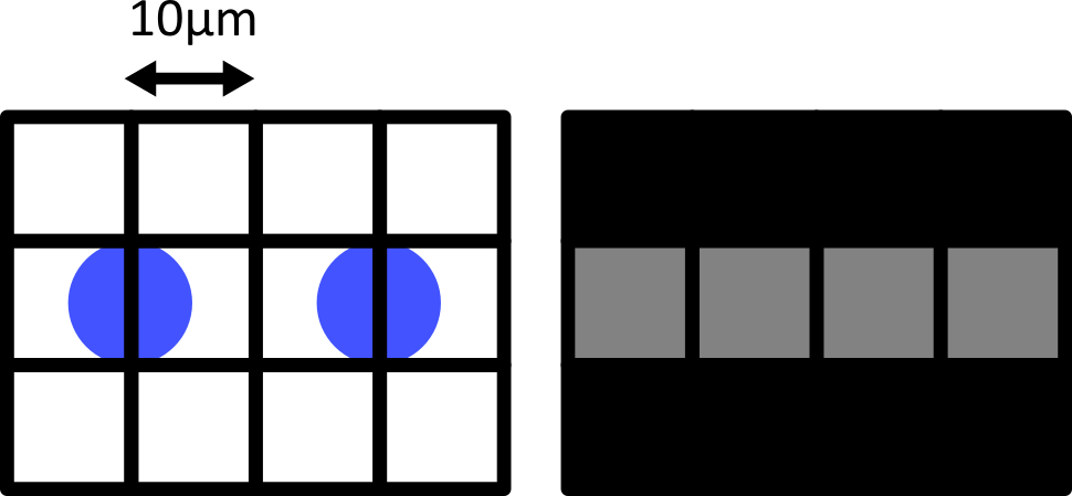
Consider the diagram below - on the left is shown two round cells (blue) that have a diameter of 10 micrometre and are overlaid by a pixel grid with the same spacing. On the right is shown the equivalent final image, using a rough grayscale colourmap (black = 0, white = maximum).
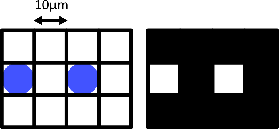
When the cells lie at the centre of each pixel, we can easily detect them as separate objects in our final image. The issue comes when the cells are offset from the pixel grid - which will happen very regularly in a real life scenario! Keeping the same 10 micrometre spacing, but offsetting the grid slightly results in a final image where where we can no longer separate the two cells:
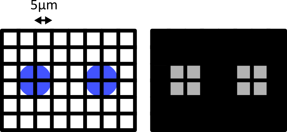
Only by decreasing the pixel size (e.g. to 5 micrometre) can we be sure to capture the two cells, no matter their alignment with the grid:
Failing to meet the Nyquist criteria can also result in various image artifacts known as ‘aliasing’. For example, consider the digram below - here we have 6 small cells (blue) that are evenly spaced in the x direction. Using a pixel spacing of 10 micrometre, this produces an odd effect in our final image, where we see a repeating pattern that is much wider than the real spacing of our cells.
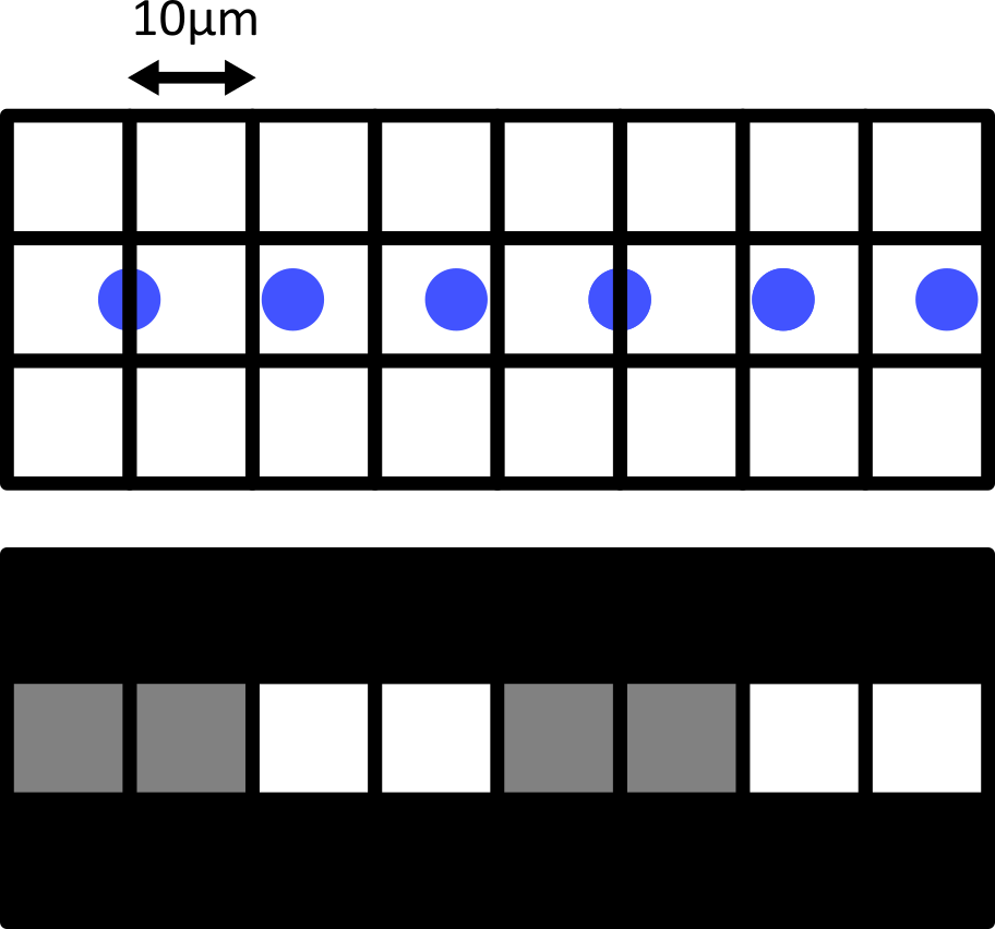
This is an example of aliasing where a high frequency detail in the image (the repeating pattern of small cells) is aliased to give a false lower frequency pattern. Aliasing and Nyquist sampling are important considerations for all fields where an analog signal is converted to a digital one - for example, digital audio and video, as well as images.
Most acquisition software will automatically provide sensible defaults that meet the Nyquist criteria (taking into account the configuration of your microscope and other acquisition settings). For example, for a laser scanning confocal, this will adjust the z-step used and the x/y spacing of points sampled with the laser. The main point is to avoid:
Undersampling: Our pixel size is too large to accurately preserve the spatial resolution in the resulting digital image (i.e. we haven’t achieved Nyquist sampling)
Oversampling: Our pixel size is too small, exceeding that required for Nyquist sampling. This results in larger images, with far more pixels, without providing any extra useful spatial information.
Initial quality control
While acquiring your images, it’s good to keep an eye on the image histogram to ensure your images are good quality. Most light microscope’s acquisition software will allow you to view a histogram in real time while imaging your sample. Recall from the image display episode that histograms provide a quick summary of pixel values in an image. This summary is a useful guide to help us adjust acquisition settings like exposure time / dwell time and laser power.
In an ideal scenario, we want our histogram to show pixel values over most of the possible intensity range. For example, for an 8-bit image, spread over most of the range from 0 (minimum) to 255 (maximum). This will ensure we are capturing as much information as possible about our sample, and giving ourselves the best chance of distinguishing features that only differ slightly in their brightness. The exercise below covers more features to look for in your image histograms, with more details in the exercise solution.
Image histogram quality control
Look at the example 8-bit image histograms below. For each:
Does it represent a good quality image, with an appropriate range of pixel values?
If not, how might you adjust your acquisition settings to improve it?
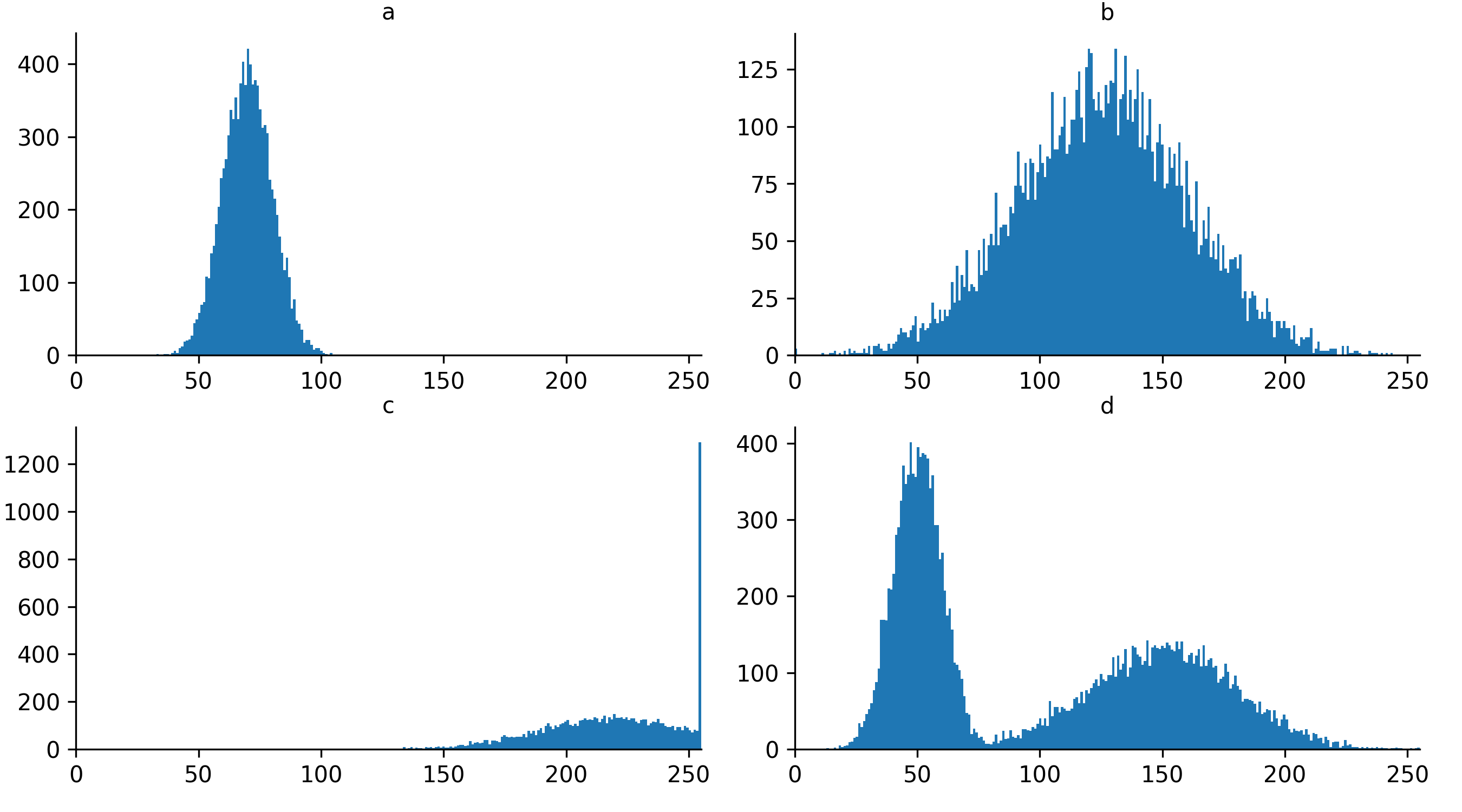
a
This image is ‘underexposed’ meaning its pixel values are clustered at low intensity values, without using much of the intensity range. As it uses such a small range of pixel values, it will be difficult to distinguish features of similar brightness.
It could be improved by increasing the amount of light collected - e.g. increasing the exposure time / dwell time or increasing light/laser power.
c
This image is ‘overexposed’ meaning its pixel values are clustered at high intensity values. It also shows ‘clipping’ (also known as ‘saturation’), as shown by the very tall peak at the right hand side of the histogram. Clipping means that some pixels are recording light above the maximum limit for the image (in this case 255). As no values beyond this limit can be recorded, they are all ‘clipped’ to the maximum value, resulting in the abnormally high peak you can see here. Clipping means that information is being irretrievably lost and should be avoided!
It could be improved by reducing the amount of light collected - e.g. reducing exposure time / dwell time or decreasing light/laser power.
Choosing acquisition settings is a trade-off between many factors including: spatial resolution, temporal resolution, field of view, data size, light exposure and signal to noise ratio.
Signal to noise ratio is a useful measure of image quality.
Magnification describes how much larger an object appears through the microscope vs its actual size. This is not the same as the spatial resolution!
Pixel size states how large a single image pixel is in physical units e.g. micrometre. Again, this is not the same as spatial resolution.
Image histograms are a useful quality control measure during acquisition. In general, we want our histogram to show pixel values spread over most of the possible intensity range.