Filetypes and metadata
Last updated on 2026-06-09 | Edit this page
Overview
Questions
- Which file formats should be used for microscopy images?
Objectives
- Explain the pros and cons of some popular image file formats
- Explain the difference between lossless and lossy compression
- Inspect image metadata with the BioIO package
- Inspect and set an image’s scale in Napari
Image file formats
Images can be saved in a wide variety of file formats. You may be familiar with many of these like JPEG (files ending with .jpg or .jpeg extension), PNG (.png extension) or TIFF (.tiff or .tif extension). Microscopy images have an especially wide range of options, with hundreds of different formats in use, often specific to particular microscope manufacturers. With this being said, how do we choose which format(s) to use in our research? It’s worth bearing in mind that the best format to use will vary depending on your research question and experimental workflow - so you may need to use different formats on different research projects.
Metadata
First, let’s look closer at what gets stored inside an image file.
There are two main things that get stored inside image files: pixel values and metadata. We’ve looked at pixel values in previous episodes (What is an image?, Image display and Multi-dimensional images episodes) - this is the raw image data as an array of numbers with specific dimensions and data type. The metadata, on the other hand, is a wide variety of additional information about the image and how it was acquired.
For example, let’s take a look at the metadata in the ‘Plate1-Blue-A-12-Scene-3-P3-F2-03.czi’ file we downloaded as part of the setup instructions. To browse the metadata we will use the BioIO package, along with its corresponding napari plugin: napari-bioio-reader. BioIO allows a wide variety of file formats to be opened in python and Napari that aren’t supported by default. BioIO was already installed in the setup instructions, so you should be able to start using it straight away.
Let’s open the ‘Plate1-Blue-A-12-Scene-3-P3-F2-03.czi’ file by
removing any existing image layers, then dragging and dropping it onto
the canvas. If a pop-up menu appears, select ‘BioIO Reader’. Note this
can take a while to open, so give it some time! Alternatively, you can
select in Napari’s top menu-bar:File > Open File(s)...
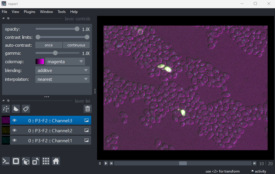
This image is part of a published dataset on Image Data Resource (accession number idr0011), and comes from the OME sample data. It is a 3D fluorescence microscopy image of yeast with three channels (we’ll explore what these channels represent in the Exploring metadata exercise).
In this case, Napari hasn’t automatically recognised the three channels - so it is loaded as one combined image layer. Recall that we looked at how Napari handles channels in the multi-dimensional images episode.
To split the image into its individual channels, and to browse its
metadata, let’s explore with BioIO in napari’s console.
Open the console and run:
PYTHON
from bioio import BioImage

# get the file path from the image layer
image_path = viewer.layers[0].source.path
image = BioImage(image_path)
Now we can explore some of the image’s properties:
OUTPUT
<Dimensions [T: 1, C: 3, Z: 21, Y: 512, X: 672]>BioIO always loads images as (t, c, z, y, x) - time,
then channels, then the 3 spatial image dimensions. You’ll notice this
image has a ‘time’ axis with length 1 i.e. this dataset only represents
a single timepoint.
We can browse a small summary of common metadata with:
This includes the image dimensions, the date/time the image was
acquired, as well as information about the pixel size
(pixel_size_x, pixel_size_y,
pixel_size_z). The pixel size is essential for making
accurate quantitative measurements from our images, and will be
discussed in the next section of this
episode.
Exploring metadata in the console
You can use python’s rich library to add colour-coding to make the output easier to read:
If you’d prefer not to have colour-coding, but keep the clearer formatting of one item per line - you can run this instead:
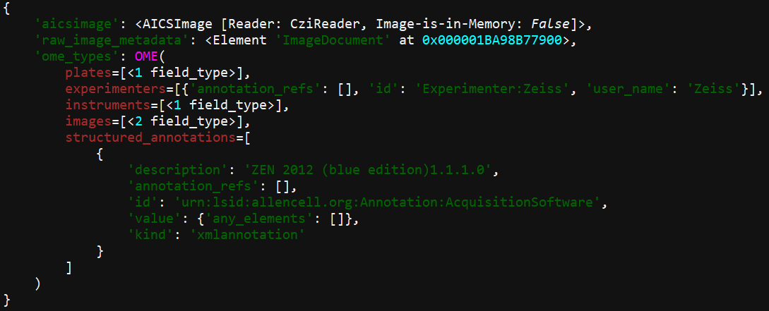
We can browse the full metadata with:
OUTPUT
OME(
    plates=[<1 field_type>],
    experimenters=[{'id': 'Experimenter:Zeiss', 'user_name': 'Zeiss'}],
    instruments=[<1 field_type>],
    images=[<2 field_type>],
    structured_annotations={
        'xml_annotations': [
            {
                'description': 'ZEN 2012 (blue edition)1.1.1.0',
                'id': 'urn:lsid:allencell.org:Annotation:AcquisitionSoftware',
                'value': {},
                'kind': 'xmlannotation'
            }
        ]
    }
)
In this case, we can see it is split into various categories
including experimenters, images and
instruments. You can look inside each of these using
.category e.g.:
The metadata is nested, so we can keep going deeper e.g.
This metadata is a vital record of exactly how the image was acquired and what it represents. As we’ve mentioned in previous episodes - it’s important to maintain this metadata as a record for the future. It’s also essential to allow us to make quantitative measurements from our images, by understanding factors like the pixel size. Converting between file formats can result in loss of metadata, so it’s always worthwhile keeping a copy of your image safely in its original raw file format. You should take extra care to ensure that additional processing steps don’t overwrite this original image.
Exploring metadata
Explore the metadata in the console to answer the following questions:
- Which manufacturer made the microscope used to take this image?
- What detector was used to take this image?
- What does each channel show? For example, which fluorophore is used?
What is its excitation and emission wavelength? (hint: look inside the
image’s pixel metadata:
metadata.images[0].pixels)
Microscope manufacturer
Under metadata.instruments[0].microscope, we can see
that the microscope manufacturer was Zeiss.
Detector
Under metadata.instruments[0].detectors, we can see that
this used an HDCamC10600-30B (ORCA-R2) detector.
Channels
Under metadata.images[0].pixels.channels, we can see one
entry per channel - Channel:1:0, Channel:2:0
and Channel:3:0.
In the first (metadata.images[0].pixels.channels[0]), we
can see that its fluor is TagYFP, a fluorophore with
emission_wavelength of 524nm and
excitation_wavelength of 508nm.
In the second (metadata.images[0].pixels.channels[1]),
we can see that its fluor is mRFP1.2, a fluorophore with
emission_wavelength of 612nm and
excitation_wavelength of 590nm.
In the last (metadata.images[0].pixels.channels[2]), we
see that no fluor, emission_wavelength or
excitation_wavelength is listed. Its
illumination_type is listed as ‘transmitted’, so this is
simply an image of the yeast cells with no fluorophores used.
BioIO image / metadata support
BioIO supports various file formats via its
different readers. During the setup
instructions, we installed the bioio-czi reader to
allow us to open the czi image for this lesson.
If you want to open more types of file, you will have to install the
relevant reader following the instructions in
the BioIO docs. Note the bioio-bioformats reader should
allow a wide range of file formats to be read.
If you have difficulty opening a specific file format with BioIO, it’s worth trying to open it in Fiji also. Fiji has very well established integration with Bio-Formats, and so tends to support a wider range of formats. Note that you can always save your image (or part of your image) as another format like .tiff via Fiji to open in Napari later (making sure you still retain a copy of the original file and its metadata!)
Pixel size
One of the most important pieces of metadata is the pixel size. In our .czi image, this is stored as:
OUTPUT
PhysicalPixelSizes(Z=0.35, Y=0.20476190476190476, X=0.20476190476190476)The pixel size states how large a pixel is in physical units i.e. ‘real world’ units of measurement like micrometre, or millimetre. In this case the unit is ‘μm’ (micrometre). This means that each pixel has a size of 0.20μm (x axis), 0.20μm (y axis) and 0.35μm (z axis). As this image is 3D, you will sometimes hear the pixels referred to as ‘voxels’, which is just a term for a 3D pixel.
The pixel size is important to ensure that any measurements made on the image are correct. For example, how long is a particular cell? Or how wide is each nucleus? These answers can only be correct if the pixel size is properly set. It’s also useful when we want to overlay different images on top of each other (potentially acquired with different kinds of microscope) - setting the pixel size appropriately will ensure their overall size matches correctly in the Napari viewer.
Let’s open the image in napari again, split by individual channels
and with the pixel size set correctly. First, remove the
Plate1-Blue-A-12-Scene-3-P3-F2-03.czi layer, then run:
PYTHON
# Get the numpy array and remove the un-needed time axis
image_np = image.data[0,]

# Display it, giving the correct 'channel_axis' to split on + pixel size
viewer.add_image(image_np, rgb=False, channel_axis=0, scale=[0.35, 0.2047619, 0.2047619])
Each image layer in Napari has a .scale which is
equivalent to the pixel size. We can check this is set correctly
with:
PYTHON
# Get the first image layer
image_layer = viewer.layers[0]

# Print its scale
print(image_layer.scale)
OUTPUT
# [z y x]
[0.35 0.2047619 0.2047619]Automatically setting scale
Depending on the BioIO reader you use, you may find that
.scale is set automatically from the image metadata when
you open it in napari (via drag and drop or
File > Open File(s)...).
It’s always worth checking the .scale property is set
correctly before making measurements from your images. You can set the
.scale of an already open image layer with:
Pixel size / scale
Copy and paste the following into Napari’s console to get
image_layer_0, image_layer_1 and
image_layer_2 of the yeast image:
PYTHON
image_layer_0 = viewer.layers[0]
image_layer_1 = viewer.layers[1]
image_layer_2 = viewer.layers[2]- Check the
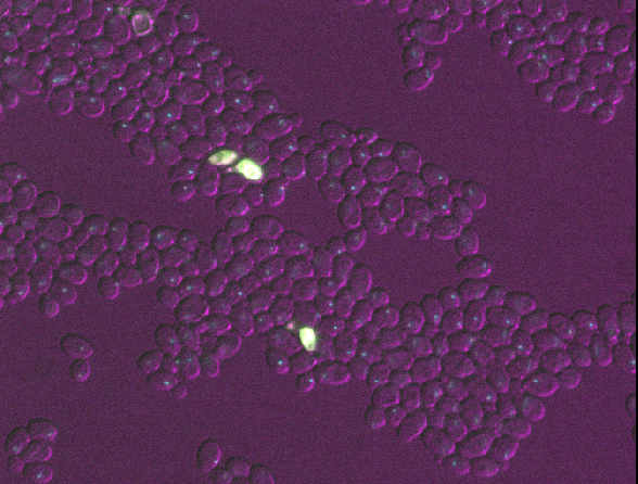
.scaleof each layer - are they the same? - Set the scale of
image_layer_2to (0.35, 0.4, 0.4) - what changes in the viewer? - Set the scale of
image_layer_2to (0.35, 0.4, 0.2047619) - what changes in the viewer? - Set the scale of all layers so they are half as wide and half as tall as their original size in the viewer
1
All layers have the same scale
OUTPUT
[0.35 0.2047619 0.2047619]
[0.35 0.2047619 0.2047619]
[0.35 0.2047619 0.2047619]
2
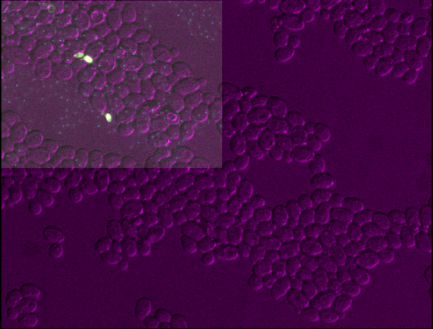
You should see that layer 2 becomes about twice as wide and twice as tall as the other layers. This is because we set the pixel size in y and x (which used to be 0.2047619μm) to about twice its original value (now 0.4μm).
3

You should see that layer 2 appears squashed - with the same width as other layers, but about twice the height. This is because we set the pixel size in y (which used to be 0.2047619μm) to about twice its original value (now 0.4μm). Bear in mind that setting the pixel sizes inappropriately can lead to stretched or squashed images like this!
Choosing a file format
Now that we’ve seen an example of browsing metadata in Napari, let’s look more closely into how we can decide on a file format. There are many factors to consider, including:
Dimension support
Some file formats will only support certain dimensions e.g. 2D, 3D, a specific number of channels… For example, .png and .jpg only support 2D images (either grayscale or RGB), while .tiff can support images with many more dimensions (including any number of channels, time, 2D and 3D etc.).
Metadata support
As mentioned above, image metadata is a very important record of how an image was acquired and what it represents. Different file formats have different standards for how to store metadata, and what kind of metadata they accept. This means that converting between file formats often results in loss of some metadata.
Compatibility with software
Some image analysis software will only support certain image file formats. If a format isn’t supported, you will likely need to make a copy of your data in a new format.
Proprietary vs open formats
Many light microscopes will save data automatically into their own proprietary file formats (owned by the microscope company). For example, Zeiss microscopes often save files to a format with a .czi extension, while Leica microscopes often use a format with a .lif extension. These formats will retain all the metadata used during acquisition, but are often difficult to open in software that wasn’t created by the same company.
Bio-Formats is an open-source project that helps to solve this problem - allowing over 100 file formats to be opened in many pieces of open source software. BioIO (that we used earlier in this episode) integrates with Bio-Formats to allow many different file formats to be opened in Napari. Bio-Formats is really essential to allow us to work with these multitude of formats! Even so, it won’t support absolutely everything, so you will likely need to convert your data to another file format sometimes. If so, it’s good practice to use an open file format whose specification is freely available, and can be opened in many different pieces of software e.g. OME-TIFF.
Compression
Different file formats use different types of ‘compression’. Compression is a way to reduce image file sizes, by changing the way that the image pixel values are stored. There are many different compression algorithms that compress files in different ways.
Many compression algorithms rely on finding areas of an image with similar pixel values that can be stored in a more efficient way. For example, imagine a row of 30 pixels from an 8-bit grayscale image:

Normally, this would be stored as 30 individual pixel values, but we can reduce this greatly by recognising that many of the pixel values are the same. We could store the exact same data with only 6 values: 10 50 10 100 10 150, showing that there are 10 values with pixel value 50, then 10 with value 100, then 10 with value 150. This is the general idea behind ‘run-length encoding’ and many compression algorithms use similar principles to reduce file sizes.
There are two main types of compression:
Lossless compression algorithms are reversible - when the file is opened again, it can be reversed perfectly to give the exact same pixel values.
Lossy compression algorithms reduce the size by irreversibly altering the data. When the file is opened again, the pixel values will be different to their original values. Some image quality may be lost via this process, but it can achieve much smaller file sizes.
For microscopy data, you should therefore use a file format with no compression, or lossless compression. Lossy compression should be avoided as it degrades the pixel values and may alter the results of any analysis that you perform!
Compression
Let’s remove all layers from the Napari viewer, and open the ‘00001_01.ome.tiff’ dataset. You should have already downloaded this to your working directory as part of the setup instructions.
Run the code below in Napari’s console. This will save a specific timepoint of this image (time = 30) as four different file formats (.tiff, .png + low and high quality .jpg). Note: these files will be written to the same folder as the ‘00001_01.ome.tiff’ image!
PYTHON
import imageio.v3 as iio
from pathlib import Path

# Get the 00001_01.ome layer, and get timepoint = 30
layer = viewer.layers["00001_01.ome"]
image = layer.data[30, :, :]

# Save as different file formats in same folder as 00001_01.ome
folder_path = Path(layer.source.path).parent
iio.imwrite( folder_path / "test-tiff.tiff", image)
iio.imwrite( folder_path / "test-png.png", image)
iio.imwrite( folder_path / "test-jpg-high-quality.jpg", image, quality=75)
iio.imwrite( folder_path / "test-jpg-low-quality.jpg", image, quality=30)
Go to the folder where ‘00001_01.ome.tiff’ was saved and look at the file sizes of the newly written images (
test-tiff,test-png,test-jpg-high-qualityandtest-jpg-low-quality). Which is biggest? Which is smallest?Open all four images in Napari. Zoom in very close to a bright nucleus, and try showing / hiding different layers with the
 icon. How
do they differ? How does each compare to timepoint 30 of the original
‘00001_01.ome’ image?
icon. How
do they differ? How does each compare to timepoint 30 of the original
‘00001_01.ome’ image?Which file formats use lossy compression?
File sizes
‘test_tiff’ is largest, followed by ‘test-png’, then ‘test-jpg-high-quality’, then ‘test-jpg-low-quality’.
Differences to original
By showing/hiding different layers, you should see that ‘test-tiff’ and ‘test-png’ look identical to the original image (when its slider is set to timepoint 30). In contrast, both jpg files show blocky artefacts around the nuclei - the pixel values have clearly been altered. This effect is worse in the low quality jpeg than the high quality one.
Lossy compression
Both jpg files use lossy compression, as they alter the original pixel values. The low quality jpeg compresses the file more than the high quality jpeg, resulting in smaller file sizes, but also worse alteration of the pixel values. The rest of the file formats (.tiff / .png) use no compression, or lossless compression - so their pixel values are identical to the original values.
Handling of large image data
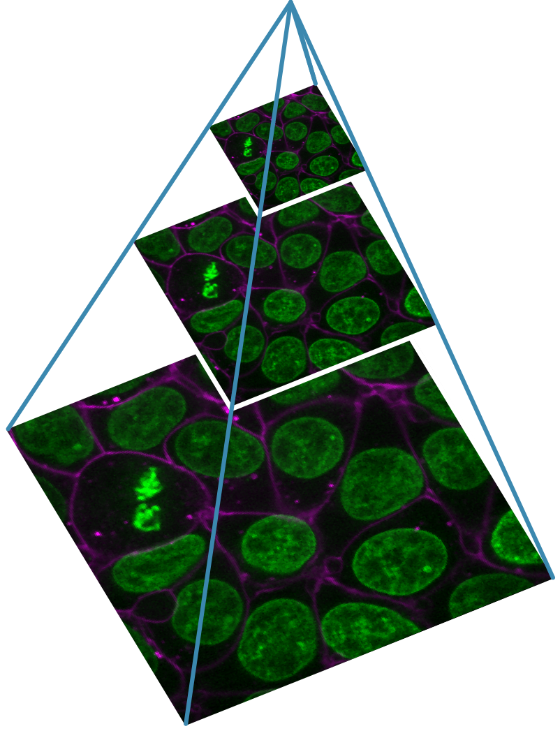
If your images are very large, you may need to use a pyramidal file format that is specialised for handling them. Pyramidal file formats store images at multiple resolutions (and usually in small chunks) so that they can be browsed smoothly without having to load all of the full-resolution data. This is similar to how google maps allows browsing of its vast quantities of map data. Specialised software like QuPath, Fiji’s BigDataViewer and OMERO’s viewer can provide smooth browsing of these kinds of images.
See below for an example image pyramid (using napari’s Cells (3D + 2Ch) sample image) with three different resolution levels stored. Each level is about twice as small the last in x and y:
Common file formats
As we’ve seen so far, there are many different factors to consider when choosing file formats. As different file formats have various pros and cons, it is very likely that you will use different formats for different purposes. For example, having one file format for your raw acquisition data, another for some intermediate analysis steps, and another for making diagrams and figures for display. Pete Bankhead’s bioimage book has a great chapter on Files & file formats that explores this in detail.
To finish this episode, let’s look at some common file formats you are likely to encounter (this table is from Pete Bankhead’s bioimage book which is released under a CC-BY 4.0 license):
| Format | Extensions | Main use | Compression | Comment |
|---|---|---|---|---|
| TIFF | .tif, .tiff | Analysis, display (print) | None, lossless, lossy | Very general image format |
| OME-TIFF | .ome.tif, .ome.tiff | Analysis, display (print) | None, lossless, lossy | TIFF, with standardized metadata for microscopy |
| Zarr | .zarr | Analysis | None, lossless, lossy | Emerging format, great for big datasets – but limited support currently |
| PNG | .png | Display (web, print) | Lossless | Small(ish) file sizes without compression artefacts |
| JPEG | .jpg, .jpeg | Display (web) | Lossy (usually) | Small file sizes, but visible artefacts |
Note that there are many, many proprietary microscopy file formats in addition to these! You can get a sense of how many by browsing Bio-Formats list of supported formats.
You’ll also notice that many file formats support different types of compression e.g. none, lossless or lossy (as well as different compression settings like the ‘quality’ we saw on jpeg images earlier). You’ll have to make sure you are using the right kind of compression when you save images into these formats.
To summarise some general recommendations:
During acquisition, it’s usually a good idea to use whatever the standard proprietary format is for that microscope. This will ensure you retain as much metadata as possible, and have maximum compatibility with that company’s acquisition and analysis software.
During analysis, sometimes you can directly use the format you acquired your raw data in. If it’s not supported, or you need to save new images of e.g. sub-regions of an image, then it’s a good idea to switch to one of the formats in the table above specialised for analysis (TIFF and OME-TIFF are popular choices).
Finally, for display, you will need to use common file formats that can be opened in any imaging software (not just scientific) like png, jpeg or tiff. Note that jpeg usually uses lossy compression, so it’s only advisable if you need very small file sizes (for example, for displaying many images on a website).
- Image files contain pixel values and metadata.
- Metadata is an important record of how an image was acquired and what it represents.
- BioIO allows many more image file formats to be opened in Napari, along with providing access to some metadata.
- Pixel size states how large a pixel is in physical units (e.g. micrometre).
- Compression can be lossless or lossy - lossless is best for microscopy images.
- There are many, many different microscopy file formats. The best format to use depends on your use-case e.g. acquisition, analysis or display.