FastSurfer
Table of contents
Now that your images are in a suitable format we can use FastSurfer on them.
Do the following:
- Run FastSurfer on all your T1 scans using the XNAT Container Service
- Look at and understand the outputted results
What is FastSurfer?
We’ll be using FastSurfer, which is a deep-learning implementation of the FreeSurfer pipeline that allows us to conduct volumetric and surface-based analysis in a much shorter timeframe than FreeSurfer itself.
Running FastSurfer with the Container Service
This is where we start to see the real benefits of using the XNAT Container Service. Usually you would have to install and configure FreeSurfer yourselves and be limited to your local machine’s performance in running the processing. However we’re using a pre-set up container that is running on a GPU-enabled server - which means everything is already set to go and allows us to use FastSurfer with GPU support. This should allow us to perform volumetric analysis and surface-based thickness analysis in relatively short timeframes.
There is one additional pre-processing step that needs to be done. All the T1 images in the iBASH study cover a Field of View (FOV) that is greater than 256mm. They also have voxel resolutions of 1.1mm. FreeSurfer likes images to be 256x256x256 with 1mm isotropic resolition. So first we must conform the Nifti files to this.
To conform the Nifti into a FS-compatible input, you must run a container in a similar manner to dcm2niix:
- Go to your project
- Go to “Project Settings” in the “Actions” menu
- Go to “Container Service -> Configure Commands”
- Enable the “Converts NIFTI to 256 conformed MGZ file” command
- Go to an imaging session in your project
- Using the “Run” on the right hand side, convert any T1 NIfTI scan
- A dialog will pop up with runtime options. Please make sure
--cw256is entered into the MRICONVERTARGS field.
As with dcm2niix, you can monitor the processing from the “History” panel at the bottom of the imaging session page. Once complete, an MGZ (a file format often used by FreeSurfer) Resource will be created at the scan level.
Then, to run FastSurfer:
- Go to your project
- Go to “Project Settings” in the “Actions” menu
- Go to “Container Service -> Configure Commands”
- Enable the “Runs FastSurfer pipeline on a conformed T1 MGZ” command
- Go to an imaging session in the project that you wish to run FastSurfer on.
- In the action menu on the right hand side fo the session page, please select the Run Container’s action and click on the “Runs FastSurfer…” container.
- A dialog runtime box will come up. please make sure to enter
--parallelin the FASTSURF_ARGS field.
Interpreting Output
You can confirm that FastSurfer has successfully completed by looking at the bottom of the page of the session that you launched the container from. There should be one line in the history with Status of Complete and Name of “FastSurfer”. It would be helpful to look at the results from teh pipeline in order to make sure that FastSurfer produced reasonable output. There are a few ways of doing this:
- Go to “Manage Files” in the action menu of the right hand side of session page. It should open up a new box that provides a tree-like structure of the underlying file data.
- Uncheck everything except for the entry called FASTSURFER and click “Download” at the bottom of the window.
- Your browser will now download a zip file.
- Alternatively, you could script this download as you may have done in previous parts of this project.
- The easiest way to view the images would likely be via FreeView, FreeSurfer’s packaged image viewer, or fsleyes, the viewer from the FSL package. If either of those will be difficult to use, please let the course leads know.
- In the viewer, select the
nu.mgzfile from the mri subdirectory and theaparc.DKTatlas+aseg.deep.mgzfrom the same directory. - Temporarily turn off the second image (
aparc.DKTatlas+aseg.deep.mgz) so that you can first check that the volumetric T1 scan (nu.mgz) is of good quality and that there is limited motion or other artefact that might make the pipeline unreliable. From this scan, you can see that the cortical boundaries could be more distinct, but it should be alright.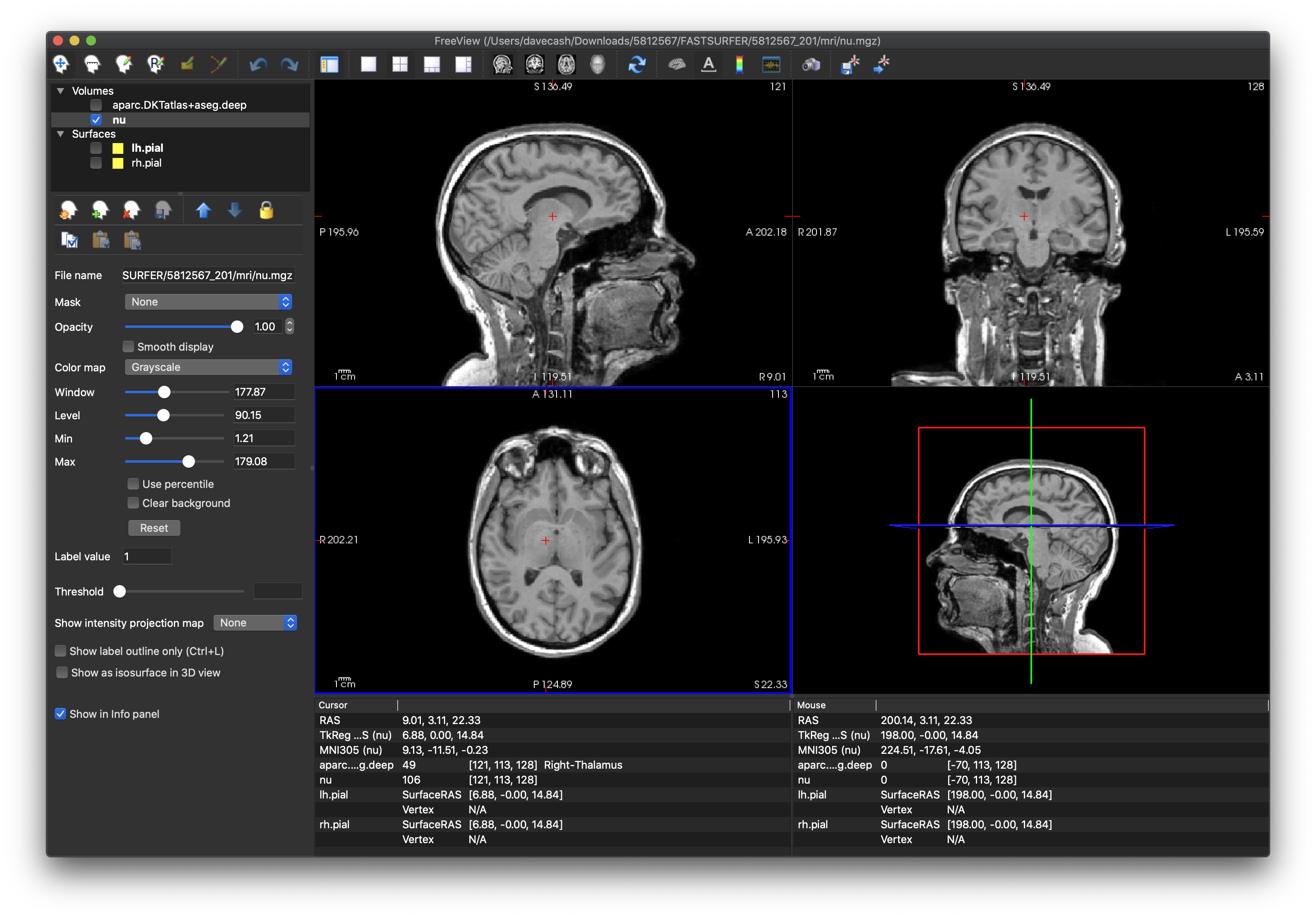
- Next, turn
aparc.DKTatlas+aseg.deep.withCC.mgzback on and select the colour map called “Lookup Table”, Make sure that the white matter is white and that the the coloured areas correspond to various parts of the cortical ribbon.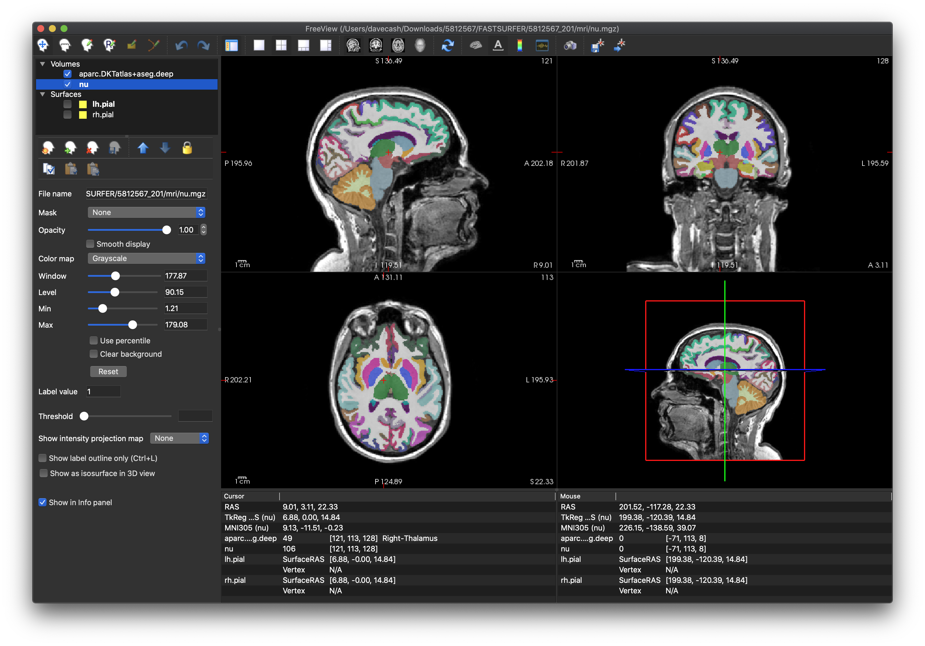
- Another way to review is to load the
lh.pialandrh.pialsurface files (from the surf subdirectory) and thenu.mgzimage volume again from above. The yellow curves representing the (left/right) hemisphere’s surface should closely adhere the boundary of the grey matter and the CSF.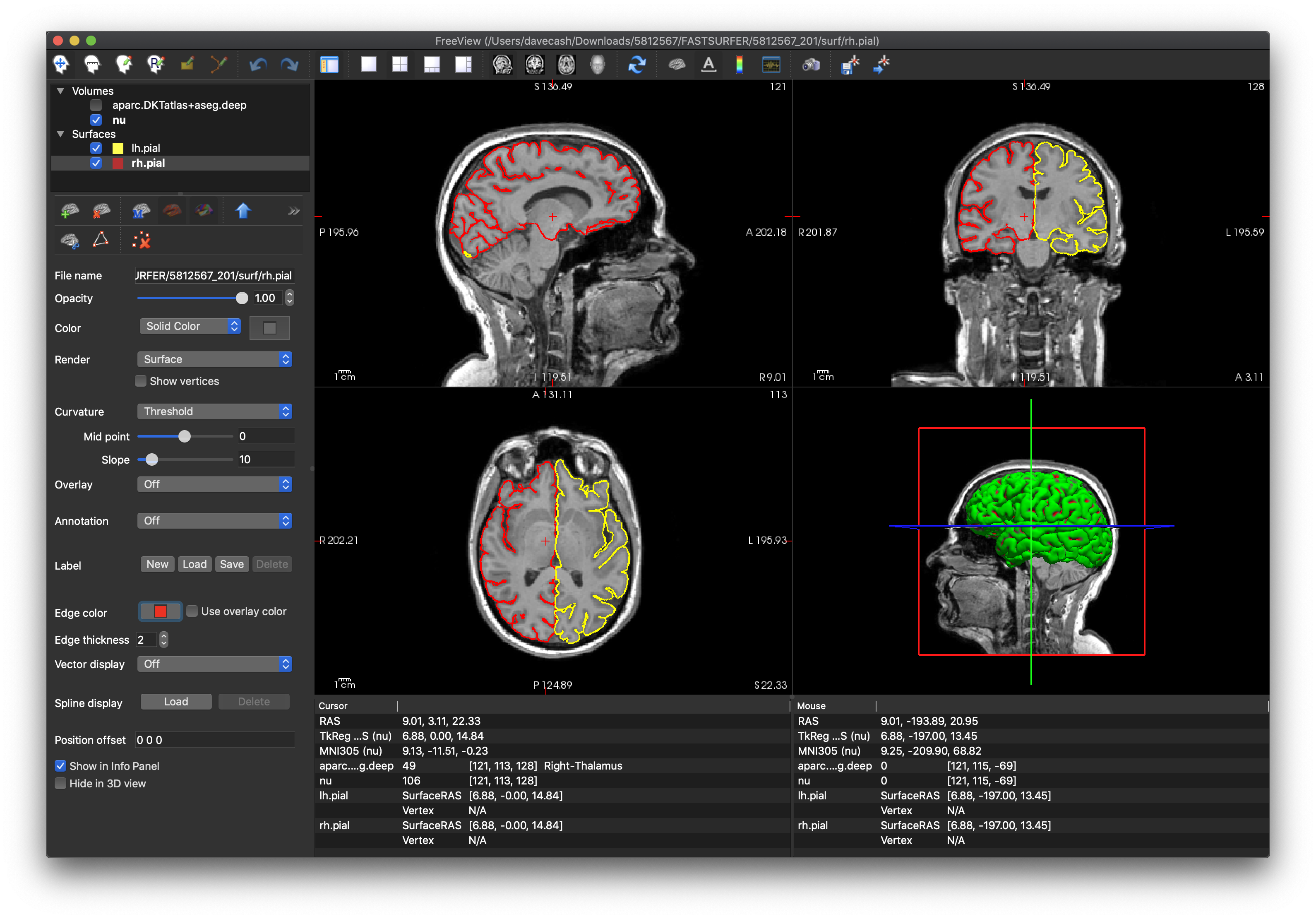
More detail of quality checking FastSurfer can be taken from this tutorial. There are also QA Tools available as part of this package if you would like to explore these as an option.
Once you have visually reviewed the data, the next step is to grab statistics. The file you want is in the stats subdiretory of the FASTSURFER resource, and it is called aseg+DKT.stats. The key part of the sample format is below.
# ColHeaders  Index SegId NVoxels Volume_mm3 StructName normMean normStdDev normMin normMax normRange
  1   2    277731   281844.1  Left-Cerebral-White-Matter       106.2308     6.4114    41.0000   131.0000    90.0000
  2   4     13034    13776.2  Left-Lateral-Ventricle            37.4730     7.3857    22.0000    73.0000    51.0000
  3   5       498      609.3  Left-Inf-Lat-Vent                 56.8333    10.7469    31.0000    83.0000    52.0000
  4   7     18989    19893.1  Left-Cerebellum-White-Matter     108.0617     7.6360    59.0000   129.0000    70.0000
  5   8     65539    65687.7  Left-Cerebellum-Cortex            90.8048    13.9321    27.0000   126.0000    99.0000
  6  10      6715     6360.5  Left-Thalamus-Proper              99.4649    10.2114    48.0000   118.0000    70.0000
  7  11      2732     2697.0  Left-Caudate                      86.3964    10.5292    54.0000   102.0000    48.0000
  8  12      4736     4780.5  Left-Putamen                      97.6617     4.2558    66.0000   108.0000    42.0000
  9  13      1994     1948.2  Left-Pallidum                    109.7849     3.7602    86.0000   124.0000    38.0000
Use your favorite tools to parse these text files and load them in your favorite software application to collate the data from multiple subjects and do some statistical analysis. You’ll look at these results again, once you have defaced the image in the next step.