Image Segmentation: Basic Concepts

Overview

Questions

• How do we perform instance segmentation in Napari?
• How do we measure cell size with Napari?

Objectives

• Use simple operations (like erosion and dilation) to clean up a segmentation.
• Use connected components labelling on a thresholded image.
• Calculate the number of cells and average cell volume.
• Save and edit your workflow to reuse on subsequent images.
• Perform more complex cell shape analysis using scikit-image’s regionprops.

Introduction

---

Now that we are able to do basic operations in Napari, let’s start doing something more applicable by segmenting some cells and measuring key properties about them.

Let’s create another notebook that we made from the last lesson and call it instance_segmentation.ipynb

Let’s import napari and open up a viewer as we did last time.

PYTHON

# Import the napari package into the notebook
import napari

# Start the viewer
viewer = napari.Viewer()

#Load in the cells image
viewer.open_sample("napari", "cells3d")

What is segmentation?

---

In order to count the number of cells, we must ‘segment’ the nuclei in this image. Segmentation is the process of labelling each pixel in an image e.g. is that pixel part of a nucleus or not? Segmentation comes in two main types - ‘semantic segmentation’ and ‘instance segmentation’. In this section we’ll describe what both kinds of segmentation represent, as well as how they relate to each other, using some simple examples.

Semantic segmentation

---

In a semantic segmentation, pixels are grouped into different categories (also known as ‘classes’). In this example, we are going to use classic image processing techniques to assign each pixel in the imate to one of two classes: nuclei or background. Importantly, it doesn’t recognise which pixels belong to different objects of the same category - for example, here we don’t know which pixels belong to individual, separate nuclei. This is the role of ‘instance segmentation’ that we’ll look at next.

This episode uses classic image processing techniques to perform the segmentation. If you would like to find more, please check out the extra Filtering and Thresholding episode.

First, we will blur the image using a Gaussian kernel. You can play with how much the images is blurred by adjusting sigma property in the gaussian function.

PYTHON

# Create a semantic segmentation 

# Import the functions we need from scikit-image
from skimage.filters import threshold_otsu, gaussian

# Access the nuclei channel from the viewer
image = viewer.layers["nuclei"].data

# Smooth the image
blurred = gaussian(image, sigma=3)

# Add the image to the viewer
viewer.add_image(blurred)

# Compute a threshold
threshold = threshold_otsu(blurred)

print("The threshold picked is:", threshold) 

OUTPUT

The threshold picked is: 0.1407702761280905

If you do pick a different blurring kernel, it might have a knock on effect on the threshold that the Otsu method chooses.

Using our threshold on the blurred image we create a semantic segmentation.

PYTHON

# Create a semantic segmentation 
semantic_seg = blurred > threshold

# Add as a labels layer to the viewer
viewer.add_labels(semantic_seg)

OUTPUT

<Labels layer 'semantic_seg' at 0x1f157459820>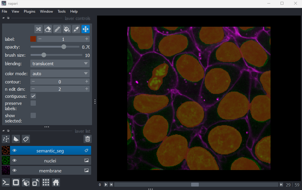

In the Napari viewer you should see the image above. Mouse over the pixels and check their intensity. You should notice that the pixels assigned to background are assigned to 0 and the pixels categorized as nuclei are have a value of 1.

Instance segmentation

---

Now we will go about creating an ‘instance segmentation’ for this image. Instance segmentations recognise which pixels belong to individual ‘instances’ of our category (nuclei). This is the kind of segmentation we will need in order to count the number of nuclei (and therefore the number of cells) in our image.

Note that it’s common for instance segmentation to be created by first making a semantic segmentation, then splitting the resulting category from the semantic segmentation into individual instances. This isn’t always the case though - it will depend on the type of segmentation method you use.

We will use the the label function from scikit-image to create an instance segmentation.

The label function is an example of connected component analysis. Connected component analysis will go through the entire image, determine which parts of the segmentation are connected to each other and form separate objects. Then it will assign each connected region a unique integer value.

PYTHON

# Instance segmentation

# Import the label function
from skimage.measure import label

# Run the label function on the mask image
instance_seg = label(semantic_seg)

# Add the result to the viewer
viewer.add_labels(instance_seg)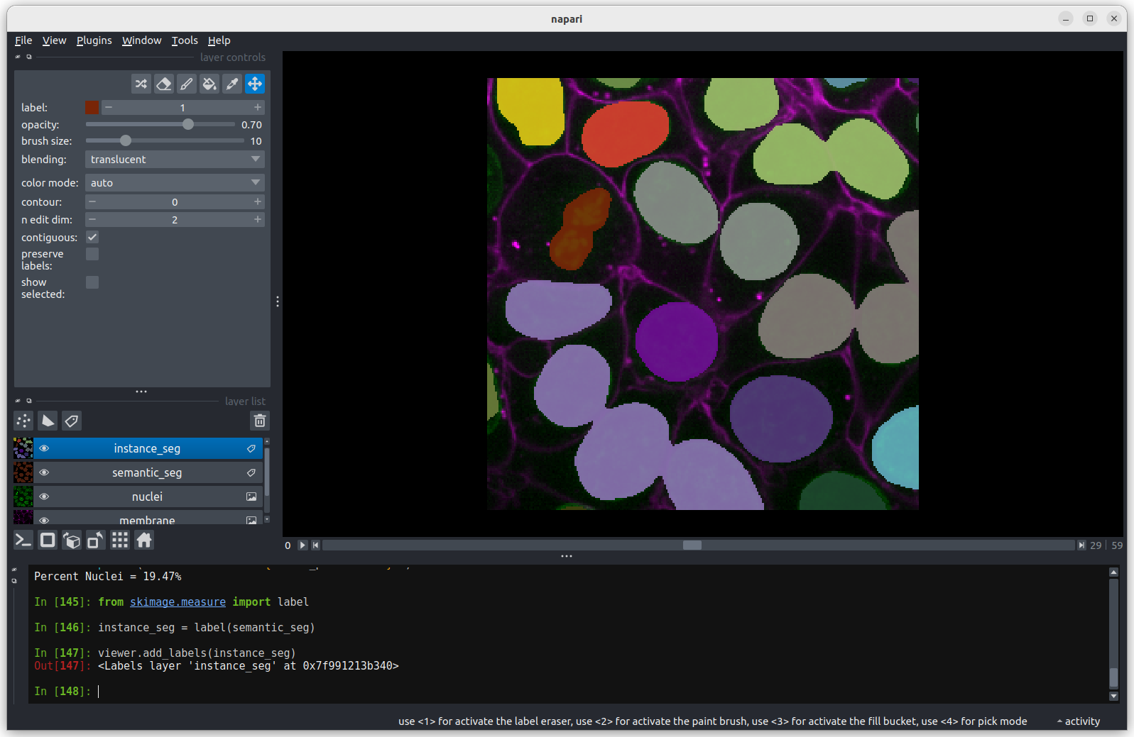

You should see the above image in the Napari viewer. The different colours are used to represent the labels of separate objects. Again, mouse over the image and notice the change of pixels. The background pixels are still assigned to 0, but each instance of the nuclei has a different label value, which has a different color assigned to that value.

Counting the nuclei

---

Because the instance segmentation assigns a different integer value starting at 1 and increasing in steps of 1 (1, 2, 3, …) to each object, counting the number of nuclei can be done very easily by taking the maximum value of the instance segmentation image.

PYTHON

# Count the nuclei
number_of_nuclei = instance_seg.max()
print("Number of nuclei: ", number_of_nuclei)

OUTPUT

Number of nuclei: 18

Using napari-skimage plugin to measure nuclei size

---

In the napari toolbar, open Layers > Measure > Regionprops (labels) (skimage). You should see a dialog like this: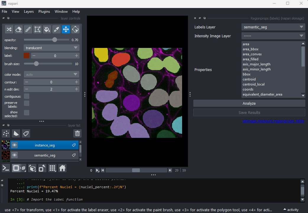

Select instance_seg in the ‘Labels layer’ drop down box and nuclei in the ‘Intensity Image Layer’ drop down box. You can choose to measure various shape properties with this plugin but for now let’s keep it simple, making sure that only area, centroid and label are selected. You will need to hold down ctrl (or ⌘ on Mac) to select multiple items in the list.

Click Analyze - a table of numeric values should appear in napari. If it opens in an inconvenient location, you can click and drag on the header containing the x, and other icons next to the table window to reposition it.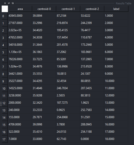

Regionprops

---

Before, we used the napari‑skimage plugin to create a table with properties of the nuclei. The same properties can also be computed using scikit-image directly in our notebook.

PYTHON

# Create a Regionprops table

# Import tools
from skimage.measure import regionprops_table
import pandas as pd

# Compute region properties
props = regionprops_table(
    label_image=instance_seg,
    properties=["label", "area", "centroid"]
)

# Convert to a pandas DataFrame
props_df = pd.DataFrame(props)

# Display the table
props_df

Sorting and inspecting the results

---

Regionprops can generate a lot of information on the shape and size of each connected region. For now we will focus only on the column headed area, which shows the size in pixels.

Let’s sort our table so that it is easier to see the extreme values.

PYTHON

# Sort the table based on cell size (area)
sorted_props_df = props_df.sort_values("area")

# Display the table
sorted_props_df

OUTPUT

    label      area  centroid-0  centroid-1  centroid-2
0       1   43945.0   39.089407   87.218409   53.622232
1       2   27187.0   33.299555  219.697392  244.239931
2       3  202258.0   34.401952  195.413526   76.441688
3       4   47652.0   34.303828  157.445417  110.678712
4       5   54018.0   31.364397  201.457755  173.293958
5       6  113935.0   36.186343   37.206205  183.966147
6       7   79226.0   33.722503   85.528072  137.286535
7       8  102444.0   34.497628  136.998624  215.951993
8       9   34421.0   35.555271   18.081346   24.130676
9      10   35227.0   34.429500   32.455418   80.085531
10     11   14525.0   31.464578  246.703408  207.343477
11     12    3258.0   35.920810    2.583487   80.581338
12     13    2000.0   32.342000  187.727500    1.962500
13     14     240.0   33.233333    0.962500  252.758333
14     15     155.0   29.787097  254.696774   51.258065
15     16    4709.0   39.099809    3.779996  208.094500
16     17     522.0   35.431034   24.015326  254.118774
17     18       7.0   33.000000   62.714286    0.000000

The largest nucleus

According to the table, nucleus 3 is larger than the other nuclei (202258 pixels). In the what is an image lesson, we learnt to use the mouse pointer to find particular values in an image. Hovering the mouse pointer over the light purple nuclei at the bottom left of the image we see that these apparently four separate nuclei have been labelled as a single nucleus.

In the layer controls of the instance_seg layer we can confirm this by selecting label 3 and enabling show selected.

Challenge

Why Are Separate Nuclei Getting the Same Label?

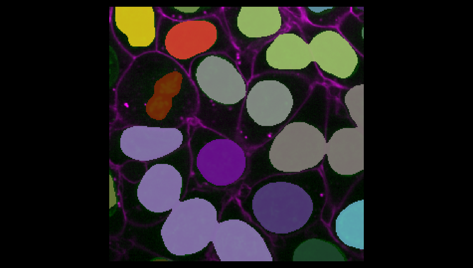
In the image above, three of the light purple nuclei are visibly touching, so it is not surprising that they have been considered as a single connected component and thus labelled as a single nucleus. What about the fourth apparently separate nucleus? Why does it have the same label?

Show me the solution

It is important to remember that this is a three-dimensional image and so pixels will be considered as “connected” if they are adjacent to another segmented pixel in any of the three dimensions (and not just in the two-dimensional slice that you are looking at).

You may remember from our first lesson that we can change to 3D view mode by pressing the button. Try it now.

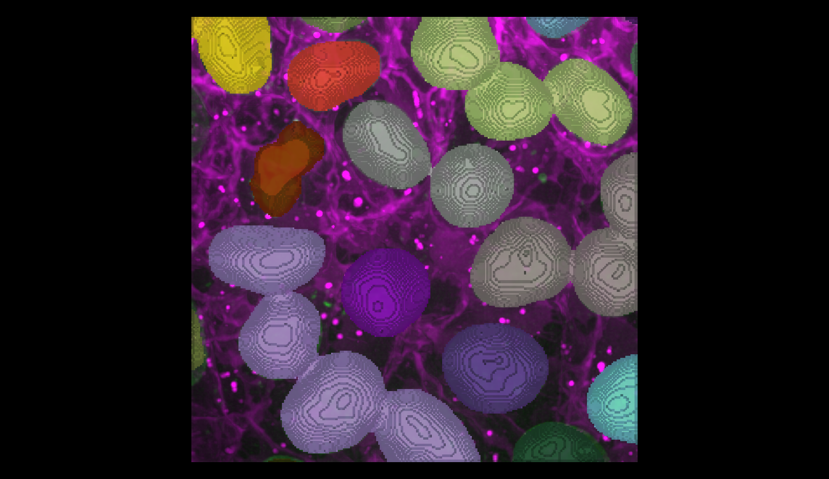You should see the image rendered in 3D, with a clear join between the upper most light purple nucleus and its neighbour.

The smallest nucleus

The smallest nucleus is labelled 18, with a size of 7 pixels. We can use the position data (the centroid columns) in the table to help find this nucleus. We need to navigate to slice 33 and get the mouse near the top left corner (33 63 0) to find label 18 in the image.

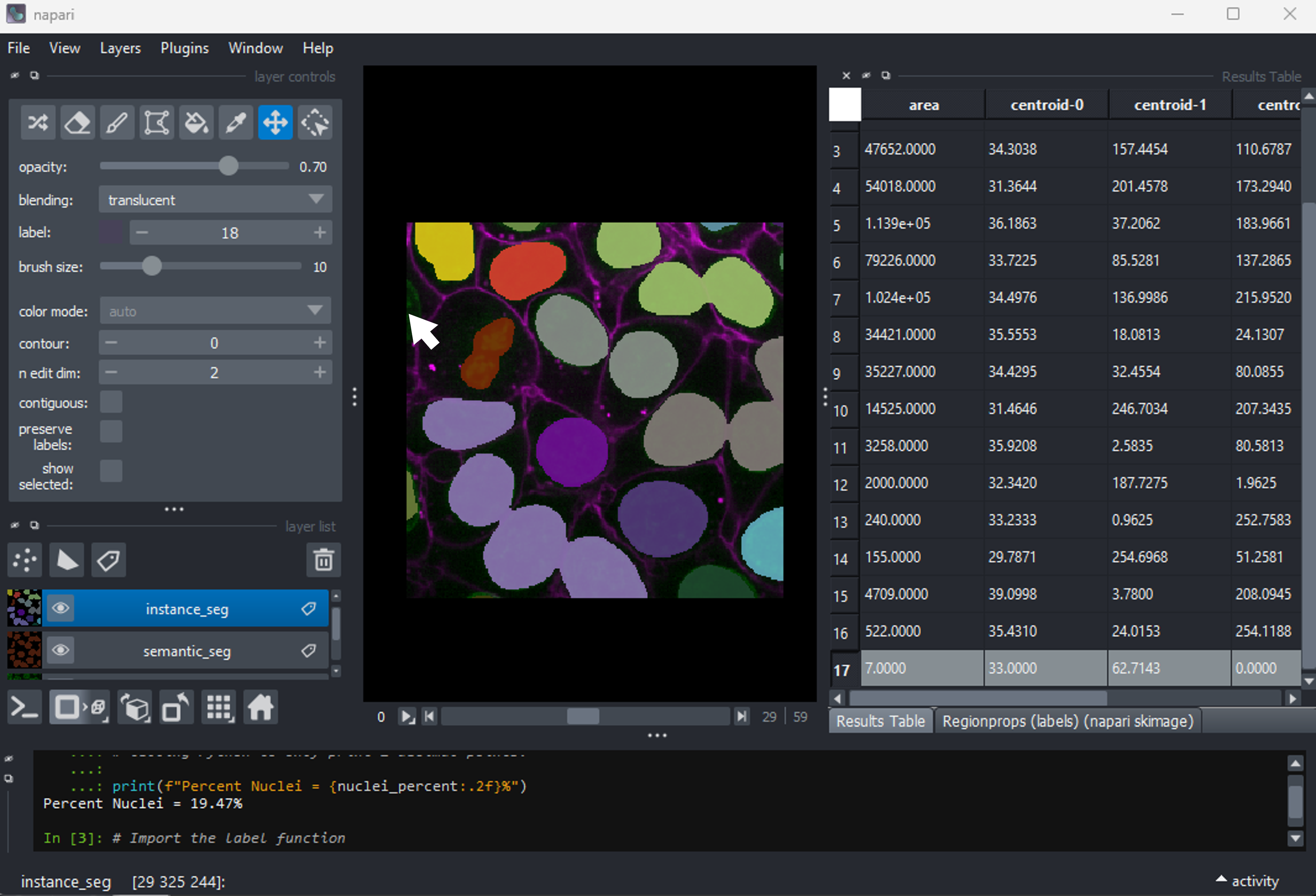
Nucleus 18 is right at the edge of the image, so is only a partial nucleus. Partial nuclei will need to be excluded from our analysis. We’ll do this later in the lesson with a clear border filter. However, first we need to solve the problem of joined nuclei.

Separating joined nuclei

---

Our first problem is how to deal with four apparently distinct nuclei (labelled with a light purple colour) being segmented as a single nucleus.

Erosion

To separate our nuclei, we can ‘erode’ our segmentation. Erosion is a type of filter, similar to those we covered in the filters and thresholding episode. It will make all segmented nuclei smaller, by setting pixels at their edge to zero.

The size / shape of the region that gets set to zero is controlled by the filter’s ‘footprint’. We’ll use scikit-image’s ball function to generate a sphere to use as the footprint. Any pixels closer to the edge of the nucleus than the radius of this sphere will be set to zero.

Create a new cell and run:

PYTHON

# Erode the semantic segmentation

# import tools
from skimage.morphology import erosion, ball

# Erosion with a radius 1 ball
eroded_mask = erosion(semantic_seg, footprint = ball(1))
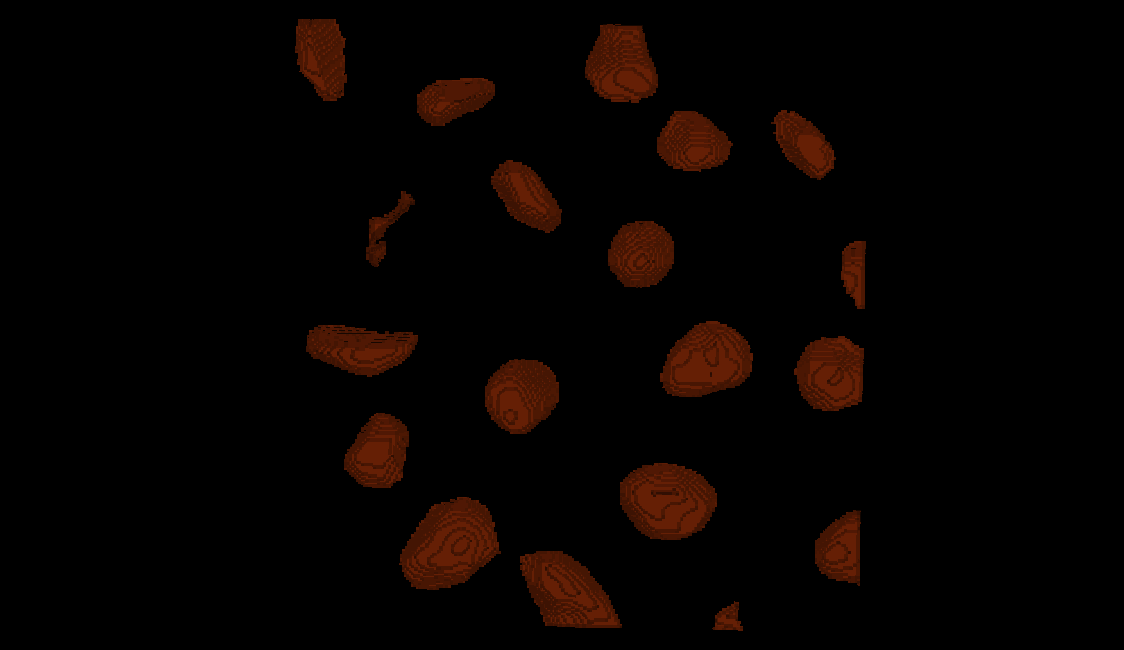
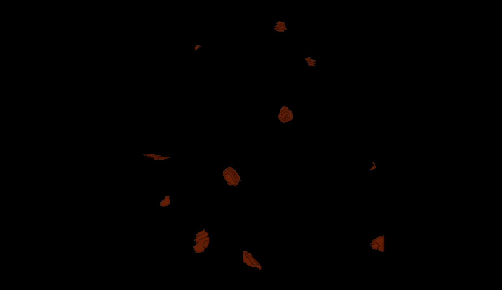
viewer.add_labels(eroded_mask, name = "eroded_ball_1")

Challenge

What is a good radius?

We can change the radius of the footprint to control the amount of erosion.

Try eroding the semantic_seg layer with different integer values for the radius. What radius do you need to ensure all nuclei are separate?

Note that larger radius values will take longer to run on your computer.

Keep your radius values <= 15.

Show me the solution

To test different values of radius, you can assign a different value to radius, e.g. radius = 5 and rerun the last two lines from above. Or you can try with a Python for loop which enables us to test multiple values of radius quickly.

PYTHON

# Erode the mask using a ball

# Radius 5
eroded_mask = erosion(semantic_seg, footprint=ball(5))
# Add the eroded mask as a new layer in Napari
viewer.add_labels(eroded_mask, name="eroded_ball_5")

# Radius 10
eroded_mask = erosion(semantic_seg, footprint=ball(10))
# Add the eroded mask as a new layer in Napari
viewer.add_labels(eroded_mask, name="eroded_ball_10")

# Radius 15
eroded_mask = erosion(semantic_seg, footprint=ball(15))
# Add the eroded mask as a new layer in Napari
viewer.add_labels(eroded_mask, name="eroded_ball_15")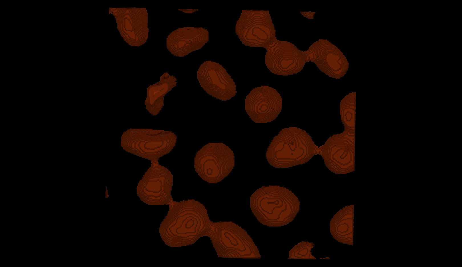

Radius 5

Some nuclei that are touching remain partially connected.

Radius 10

Erosion with a radius of 10 removes enough pixels to separate touching nuclei
while still keeping the nuclei you want to analyse.

Radius 15

Erosion with a radius of 15 is too strong: several nuclei become over‑eroded
and some disappear completely.

Challenge

For-loop to test different radii

Try using a Python for loop to test several radius values.

Show me the solution

You can change the radius manually (for example, radius = 5) and re‑run the erosion each time.
But if you want to test many radius values quickly, a Python for loop lets you repeat the same steps for each radius in a list.

PYTHON

# List of radii to test
radii = [5, 10, 15]
# A for-loop that tests several radii
for radius in radii:
    # Make a name for the output layer
    layer_name = "eroded_ball_" + str(radius)
    # Erode the mask using this radius
    eroded_mask = erosion(semantic_seg, footprint=ball(radius))
    # Add the eroded mask as a new layer in Napari
    viewer.add_labels(eroded_mask, name=layer_name)

It is also possible to run the erosion function through a plugin: Layers > Filter > Morphology > Binary Morphology (napari skimage).

Instance segmentation using the eroded mask

Now we have separate nuclei, lets try creating instance labels again.

PYTHON

# Create a new instance segmentation using the eroded mask
eroded_mask = erosion(semantic_seg, footprint=ball(10))
instance_seg = label(eroded_mask)

# Remove old instance segmentation
viewer.layers.remove('instance_seg')

# Add new instance segmentation
viewer.add_labels(instance_seg)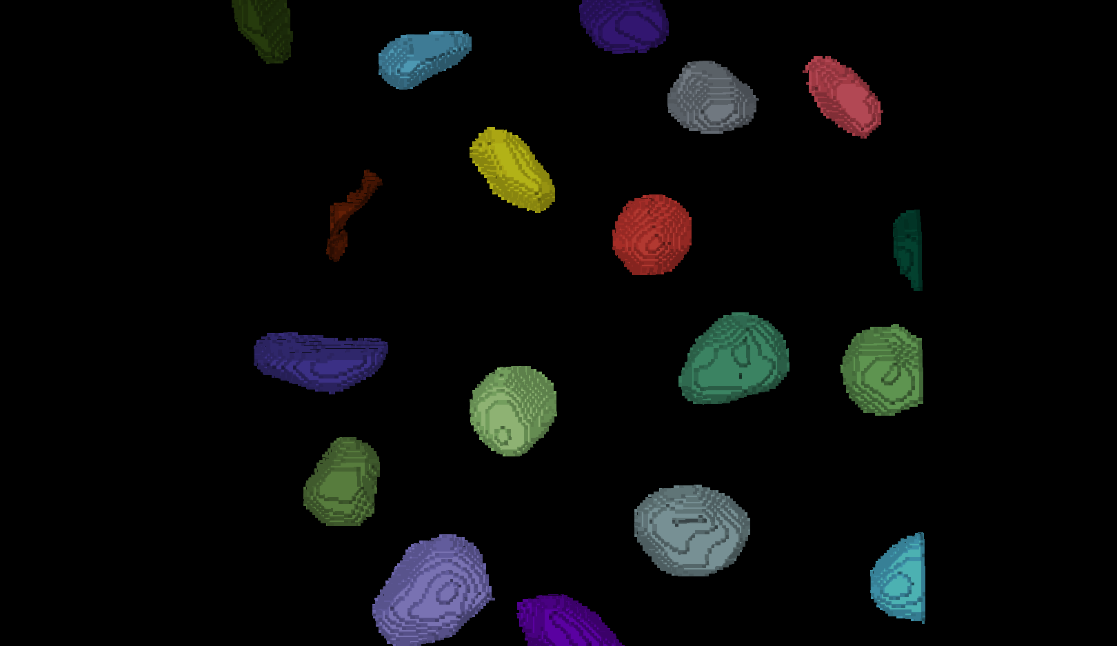

Looking at the image above, there are no longer any incorrectly joined nuclei.

Dilation

We managed to separate the nuclei, however performing any size or shape analysis on these nuclei will be flawed, as they are heavily eroded.

We can largely undo the erosion by using scikit-image’s expand labels function.

The expand labels function is a filter which performs a dilation, expanding the bright (non-zero) parts of the image. The expand labels function adds an extra step to stop the dilation when two neighbouring labels meet, preventing overlapping labels.

PYTHON

from skimage.segmentation import expand_labels

# Dilate eroded instance segmentation with the same radius
instance_seg = expand_labels(instance_seg, 10)

# Remove old instance segmentation
viewer.layers.remove('instance_seg')

# Add new instance segmentation
viewer.add_labels(instance_seg)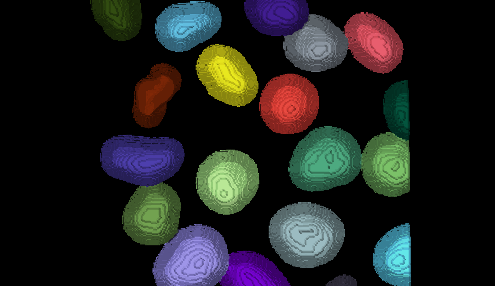

There are now 19 apparently correctly labelled nuclei that appear to be the same shape as in the original mask image.

Opening

In order to create a correct instance segmentation we have performed a mask erosion followed by a label expansion. This is a common image operation often used to remove background noise, known as as opening, or an erosion followed by a dilation. In addition to helping us separate instances it will have the effect of removing objects smaller than the erosion footprint, in this case a sphere with radius 10 pixels.

Challenge

Is the erosion completely reversible?

If we compare the eroded and expanded image with the original mask, what will we see?

Show me the solution

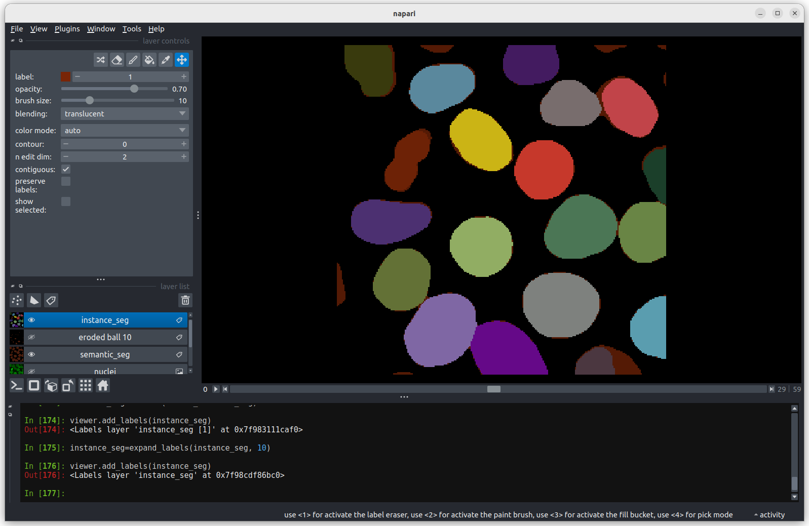Looking at the above image we can see some small mismatches around the edges of most of the nuclei. It should be remembered when looking at this image that it is a single slice though a 3D image, so in some cases where the differences look large (for example the nucleus at the bottom right) they may still be only one pixel deep. Will the effect of this on the accuracy of our results be significant?

Removing Border Cells

---

Now we return to the second problem with our initial instance segmentation, the presence of partial nuclei around the image borders. As we’re measuring nuclei size, the presence of any partially visible nuclei could substantially bias our statistics.

We can remove these from our analysis using scikit-image’s clear border function.

PYTHON

# Remove partial nuclei touching the image border

# Import scikit-image's clear_border
from skimage.segmentation import clear_border

# Clear border
instance_seg = clear_border(instance_seg)

# Remove old instance segmentation
viewer.layers.remove('instance_seg')

# Add new instance segmentation
viewer.add_labels(instance_seg)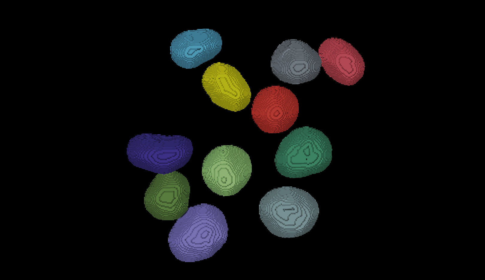

We now have an image with 11 clearly labelled nuclei. You may notice that the smaller nucleus (dark orange) near the top left of the image has been removed even though we can’t see where it touches the image border. Remember that this is a 3D image and clear border removes nuclei touching any border. This nucleus has been removed because it touches the top or bottom (z axis) of the image.

Let’s check the nuclei count as we did above.

PYTHON

# First count the nuclei
number_of_nuclei = instance_seg.max()
print("Number of nuclei: ", number_of_nuclei)

OUTPUT

Number of nuclei: 19

Why are there 19 nuclei?

When we ran clear_borders the pixels corresponding to border nuclei were set to zero, however the total number of labels in the image was not changed, so whilst there are 19 labels in the image some of them have no corresponding pixels. The easiest way to correct this is to relabel the image (and replace the old instance segmentation in the viewer.)

PYTHON

# Relabel
instance_seg = label(instance_seg)

# Remove old instance segmentation
viewer.layers.remove('instance_seg')

# Add relabeled instance segmentation
viewer.add_labels(instance_seg)

# Number of nuclei after relabling
number_of_nuclei = instance_seg.max()
print("Number of nuclei:", number_of_nuclei)

OUTPUT

Number of nuclei: 11

Number of pixels per nucleus

---

Now that your instance segmentation is correct, you can finish the analysis in our notebook.

Let’s start by counting the pixels per nucleus like we did before.

PYTHON

# Count the pixels per nucleus

# Extract region properties 
props = regionprops_table(
    instance_seg,
    properties=["label", "area"]   # 'area' = number of pixels
)

# Convert to a pandas DataFrame
props_df = pd.DataFrame(props)

props_df

Are these pixel counts useful measurements? Pixel counts depend on image resolution, rather than the real size of a biological structure. This means images of the exact same nuclei taken with different settings could give vastly different values for the number of pixels.

This is why biologists convert pixel counts into physical units like µm³ that allow comparisons across experiments, microscopes, and labs.

Volume per nuclei

---

To convert to volumes we need to know the pixel size, which tells us the physical measurement of each dimension of a pixel. This information is often stored inside the image metadata that comes with the pixel data itself.

Unfortunately the sample image we’re using in this lesson has no metadata. Fortunately the image pixel sizes can be found in the scikit-image documentation. So we can assign a pixel size of 0.26μm (x axis), 0.26μm (y axis) and 0.29μm (z axis).

Using this pixel size, we can then calculate the nucleus volume in cubic micrometres.

PYTHON

# Volume of a single voxel in cubic micrometres
voxel_volume = 0.26 * 0.26 * 0.29

# Add a physical volume column
props_df["volume_um3"] = props_df["area"] * voxel_volume

props_df

Once you know the voxel size, pandas makes the conversion and analysis extremely easy:

PYTHON

# Quick stats using pandas
props_df["volume_um3"].describe()

OUTPUT

count      11.000000
mean      855.980145
std       178.497656
min       602.391712
25%       729.190384
50%       800.019636
75%       983.473868
max      1181.493872
Name: volume_um3, dtype: float64

Key Points

• Connected component analysis (the label function) was used to assign each connected region of a mask a unique integer value. This produces an instance segmentation from a semantic segmentation.
• Erosion and dilation filters were used to correct the instance segmentation. Erosion was used to separate individual nuclei. Dilation (or expansion) was used to return the nuclei to their (approximate) original size.
• Partial nuclei at the image edges can be removed with the clear_border function.
• The napari-skimage plugin can be used to interactively examine the nuclei shapes.