Structural MRI - Bias Correction, Segmentation and Image Registration

Introduction

In this section, you will be learning how to process and quantify structural MRI scans. T1-weighted structural MRI scans are the “workhorse” scan of dementia research. They provide high-resolution, detailed pictures of a patients anatomy, allowing researchers to visualize where atrophy caused by Alzheimer’s disease or other dementias is occurring. In addition, it provides anatomical reference to other imaging modalities, such as functional MRI and positron emission tomography (PET), that provide lower resolution maps of brain function and pathology, so that regional quantification of key areas can be assessed in these scans.

We will be using FreeSurfer, a software package for the analysis and visualization of structural and functional neuroimaging data that can be used in both cross-sectional or longitudinal studies. It is a “one stop shop” that can perform a complete neuroimaging analysis of a structural MRI scan. The subsequent outputs from this pipeline can be used to aid in the quantification of other imaging modalities. It is one of the most widely used imaging analysis packages in dementia research.

After the course, you will be able to compute measures relevant to dementia research from structural MRI brain scans, such as the cortical thickness of a previously defined region of interest (Jack et al. Alzheimers Dement. 2017) or the global amyloid PET signal to establish whether a subject is amyloid-positive or negative (Mormino et al. Brain. 2009).

We will use the Freesurfer tools to perform:

image visualization of analysis outputs,
intensity inhomogeneity correction,
structural MRI segmentation, and
multimodal image coregistration.

Setting up FreeSurfer

FreeSurfer has been installed on your machine, so the first step is to define an environment variable that stores the path (or location) where all FreeSurfer output is to be stored for each of the analyzed subjects, so that Freesurfer knows where to look for the data. This variable is called SUBJECTS_DIR and the structure of the directory is:

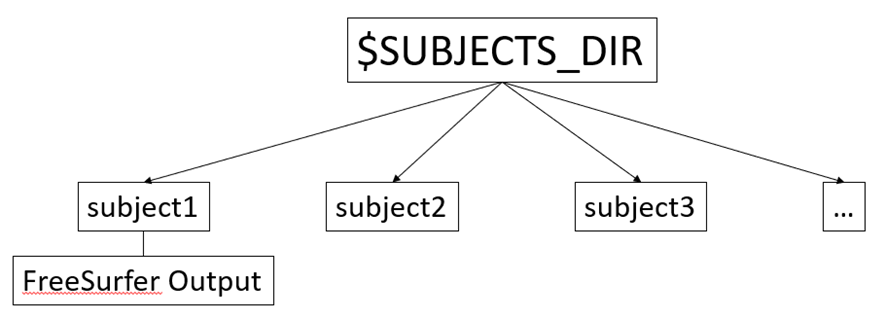
subject1, subject2, etc. are the directories in which the respective subject’s output is stored. We will go over FreeSurfer output later. By default, FreeSurfer will assign a prespecified path to SUBJECTS_DIR. You can check this path by typing:

echo $SUBJECTS_DIR

If we want to change the SUBJECTS_DIR directory, we just need to redefine the SUBJECTS_DIR variable. For this course, we have to set our SUBJECTS_DIR to the following path:

SUBJECTS_DIR=~/oasis/subjects

Remember the ~ is a shortcut to represent your home directory.

Keep in mind that every time you close and open your terminal the SUBJECTS_DIR variable will be set back to its default path (/usr/local/freesurfer/subjects).

Running FreeSurfer recon-all

Now that we have defined our SUBJECTS_DIR directory, we can run the actual FreeSurfer processing pipeline. This command is called recon-all, as it stands for reconstruction: FreeSurfer reconstructs a two-dimensional cortical surface based on the information contained in a three-dimensional T1 scan, which is the basis for cortical segmentation. The recon-all command also provides segmentations of subcortical brain structures, and it produces output files containing the relevant volumetric and morphometric measures derived from both the surface- and volume-based segmentations. While a complete analysis of a T1 scan is is performed with just a single command, recon-all typically takes anywhere from 3 to 24 hours to run depending on your computer’s hardware. As a result, we have already run this command for you so that you can examine the resulting output.

Let’s see how to run recon-all. recon-all has the following structure:

recon-all -s subject1 -i /path_to_T1_image -all

The name of the subject is provided using the -s flag. In this example it is set to subject1 but you can set to whatever value you want.
The input T1 scan to analyze is set with the flag -i .
The flag -all tells recon-all that you want to perform all the steps of the pipeline. You would usually use this option, except in some occasions where there may be a need to manually edit the outputs from recon-all and then re-run.

recon-all has several additional options that you may want to investigate to see if they are useful for analyzing your own data. You can find out more about them on your own time by reviewing documentation on the wiki and using the -help option in recon-all

recon-all -help

As previously mentioned, we have already run recon-all, but let’s look at how we used it for some real data that you will inspect. We have selected three participants from the OASIS-3 database, one cognitively normal individual (CN), one patient with Alzheimer’s (AD) and one patient with frontotemporal dementia (FTD). The T1 scans of these subjects are located in:

Path CN scan: ~/oasis/all_subjects_BIDS/OAS30015_MR_d2004/anat/sub-OAS30015_ses-d2004_T1w.nii.gz

Path AD scan: ~/oasis/all_subjects_BIDS/OAS30758_MR_d0007/anat/sub-OAS30758_ses-d0007_T1w.nii.gz

Path FTD scan: ~/oasis/all_subjects_BIDS/OAS31171_MR_d0752/anat/sub-OAS31171_ses-d0752_T1w.nii.gz

Thus, to run recon-all for, e.g., the cognitively normal individual we would just need to type

AGAIN DON’T RUN THIS COMMAND, recon-all TAKES 3-24 HOURS IN COMPLETING THE ANALYSIS. WE’VE RUN recon-all ALREADY FOR YOU.

recon-all -s CN -i ~/oasis/all_subjects_BIDS/OAS30015_MR_d2004/anat/sub-OAS30015_ses-d2004_T1w.nii.gz -all

Here, we set the subject’s name to CN (cognitively normal).

Exercise 1

What would be the corresponding recon-all command for the Alzheimer’s (assume that subject name is AD) and frontotemporal dementia (subject name is FTD) subjects? AGAIN DON’T RUN THESE COMMANDS - THEY HAVE ALREADY BEEN PERFORMED FOR YOU.

As we mentioned before, FreeSurfer’s output will be stored in the SUBJECTS_DIR directory. Type:

ls $SUBJECTS_DIR

to see the output folders of the CN, AD, and FTD subjects.

Let’s see how the output looks like for our CN subject. Type:

ls $SUBJECTS_DIR/CN

The important directories for us are

mri/: here we have all the volumes, including bias corrected scans and volumetric segmentations.
surf/: here we can find all the 2-D surface reconstructions, together with morphometric cortical maps such as maps of cortical thickness.
label/: here we have all the annotation files that label the cortical surfaces into different regions of interest.
stats/: here we can find all the necessary files to obtain quantitative metrics such as volumes, cortical thickness, or cortical area measures.

Visualizing data with Freeview

After successfully running recon-all, we will typically wish to check whether FreeSurfer has actually done a good job. For this, we will use Freeview, which is the visualization tool integrated in FreeSurfer. FreeView is very similar in functionality to the FSLeyes tool that you will use in other sections of this course. To open Freeview we will use a command with the following structure:

freeview -v /volume1 /volume2 /volume… -f /surface1 /surface2 /surface…

The flag -v is to load volumetric (3D) images; /volume1 /volume2 /volume… are the paths of the volumes we want to visualize
The flag -f is to load surfaces (2D); /surface1 /surface2 /surface… are the paths of the surfaces we want to visualize

Freeview can load several volumes and surface at one time.

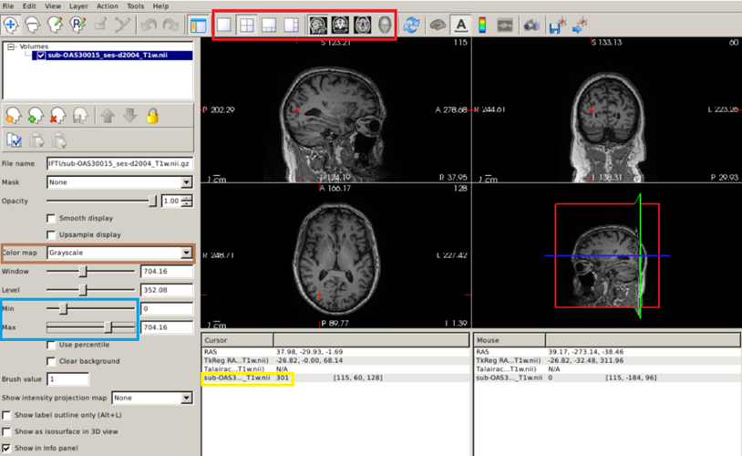
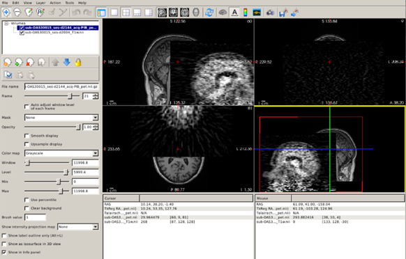
Once we have loaded our image with Freeview, we can navigate across the slices by placing the cursor over the image and use the ↑ ↓ arrow keys; to zoom in/out, use the scroll wheel; you can switch the displayed planes using the buttons highlighted by the red box in the figure below.

Exercise 2

Use Freeview to visualize the original T1 scans of our CN subject (OAS30015_MR_d2004). Click on a white matter region: the value within the yellow box below is the actual intensity value. Play with the different types of image displays (red box), with intensity saturation (blue box), and with different color maps (brown box).

Additional options for Freeview can be reviewed by typing:

freeview -help

Now that we have given you an overview of Freesurfer, the main reconstruction pipeline, and how to visualize data looking at Freeview, let’s take a look at some of the key processing steps and outputs from them to ensure Freesurfer has done a good job.

Bias correction

Magnetic resonance images often exhibit image intensity non-uniformities that are the result of magnetic field variations rather than anatomical differences. These variations are often seen as a signal gain change that varies slowly spatially. This can result in white matter voxels in one part of the brain having similar intensities to voxels with the same intensity as grey matter in other parts of the brain. However, the intensities in the white matter voxels should be more or less uniform throughout the brain. Any remaining inhomogeneity in the image can significantly influence the results of automatic segmentations, so we need to correct for these effects.

Let’s see this effect in our data. Open the original T1 scan of the CN subject with freeview:

freeview -v ~/oasis/all_subjects_BIDS/OAS30015_MR_d2004/anat/sub-OAS30015_ses-d2004_T1w.nii.gz

Let’s focus on the axial plane and scroll to superior regions of the brain. With the default gray colorscale, it may be difficult to tell whether the signal intensity actually changes. Let’s change the colormap to “NIH” and set the maximum intensity to 750.

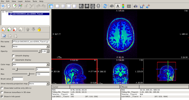
Now, the intensity changes are clear, with brighter white matter in posterior brain regions compared to anterior regions. The take-home message is that the grayscale is not the only possible color map for a T1 scan, and sometimes other color maps can be useful.

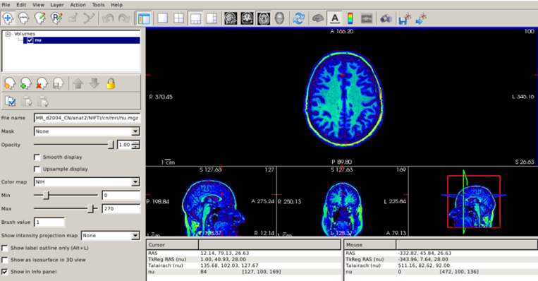
Fortunately, FreeSurfer automatically corrects for intensity inhomogeneity. The bias-corrected image can be found in the subject’s mri/ directory (its name is nu.mgz), and it is always a good idea to check that FreeSurfer has done a good job correcting for inhomogeneity.

freeview -v $SUBJECTS_DIR/CN/mri/nu.mgz

Setting the NIH colorscale and the maximum intensity to 270, we can see that the image is now much more uniform:

Inspecting cortical segmentation

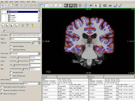
After assuring that our T1 scan has been properly corrected for intensity inhomogeneity, the next step is to inspect the results of the FreeSurfer segmentation. As mentioned before, FreeSurfer’s cortical segmentation is based on the reconstruction of surfaces, in particular the surfaces that define the boundary between white matter and gray matter (known as white surface) and the boundary between gray matter and cerebrospinal fluid (known as pial surface). Thus, it is important to make sure that these surfaces accurately follow the gray and white matter boundaries. Let’s check this for our CN subject; remember that all our surfaces are stored in the surf/ directory.

freeview -v  $SUBJECTS_DIR/CN/mri/brainmask.mgz -f $SUBJECTS_DIR/CN/surf/lh.white:edgecolor=blue $SUBJECTS_DIR/CN/surf/lh.pial:edgecolor=red $SUBJECTS_DIR/CN/surf/rh.white:edgecolor=blue $SUBJECTS_DIR/CN/surf/rh.pial:edgecolor=red

We open the brainmask.mgz volume, which represents the skull-stripped T1 scan.
lh.white and rh.white are the left and right white surfaces, respectively.
lh.pial(rh.pial) is the left (right) pial surface.
After loading each surface, we can use the : to indicate that we want to specify additional options that describe what information to display with that surface and how to display it.
After each of the pial and white surfaces have been listed, we indicate, using the edgecolor option that white surfaces are displayed as blue contours and pial surfaces as red.

To inspect surfaces, we typically navigate through slices in the coronal plane. You can hide or turn off a layer by unchecking the check box next to the layer name.

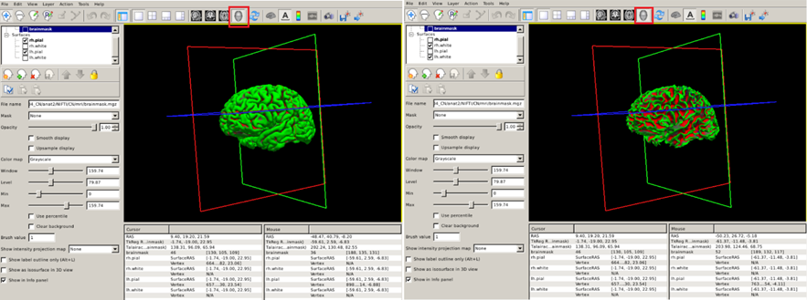
We can also visualize 3D renderings of the brain surfaces. This allows us to identify potential segmentation defects and, if the segmentation is correct, to visualize regions with potentially relevant abnormalities. For this, uncheck the brainmask.mgz and to visualize the pial (white) surfaces, uncheck the white (pial) surfaces. Select the 3D view (red box below).

Inspecting cortical parcellation

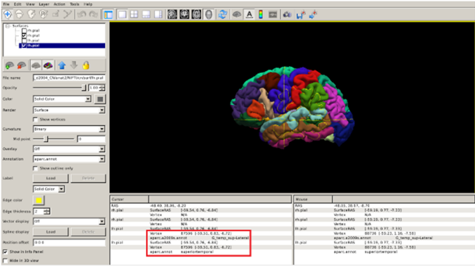
FreeSurfer also parcellates the cortex, or divides it up into smalller neuroanatomical units, assigning each surface vertex an anatomical label. There are many different protocols for performing a parcellation, but the most common in FreeSurfer, particularly for dementia research, is based on the Desikan-Killiany (DK) atlas. This parcellation is stored in the label/ directory within your subject’s directory. The Freeview command to visualize the DK parcellation on top of the cortical surface is the following:

freeview -f $SUBJECTS_DIR/CN/surf/lh.pial:annot=aparc.annot $SUBJECTS_DIR/CN/surf/rh.pial:annot=aparc.annot --viewport 3d

The annot option for a surface tells FreeSurfer to paint colours on the pial surface based on what label the parcellation has provided.
The --viewport 3d option is simply to automatically set the 3D rendering view that you saw in the previous visualisation.

You can check the name of the region by clicking on it (red box below).

Exercise 3

Repeat the previous steps to visualize the cortical parcellation of the FTD subject.

Labels are not the only thing we can overlay on the cortical surface. For further surface based visualization, please see the Stretch Your Knowledge section.

Volumetric segmentation

Now, we will go over the main volumetric segmentation output from FreeSurfer, often referred to as the aparc+aseg segmentation. This segmentation contains cortical and subcortical regions of interest. The DK atlas based aparc+aseg is commonly used in dementia research, for example in the quantification of tau and amyloid PET scans (Jack et al. Alzheimers Dement. 2017; Mormino et al. Brain. 2009).

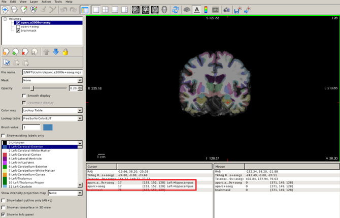
Let’s visualize these segmentations with Freeview. Segmentations are 3D images, where the voxel value represents which anatomical label is assigned. Loading these volumes on top of the T1 can be done in Freeview with the following:

freeview -v $SUBJECTS_DIR/CN/mri/brainmask.mgz $SUBJECTS_DIR/CN/mri/aparc+aseg.mgz:colormap=lut:opacity=0.2 

Just like with surfaces, we can provide additional information on how to display the volumes by adding a : after the filename.
We select the Look Up Table, or lut, colormap which sets a different color for each value in the volume (thus it’s useful for visualizing segmentations).
We set the opacity option to 0.2 to simultaneously visualize the skull-stripped T1 scan.

By clicking on the different regions of interest we can get the region name (red box below):

Obtaining quantitative morphometric and volumetric measures

Key measurements that can be extracted from a T1 scan in the context of dementia are quantitative metrics that describe the degree of atrophy in a specific brain region. These metrics can be the volume of the region of interest (e.g. the volume of the left hippocampus or the volume of the entorhinal cortex) or the average thickness of a cortical structure (e.g the precuneus). Though volumetric and thickness measures describe essentially the same pathological process, thickness metrics may be more sensitive for describing atrophy in the cortex.

Let’s see how to obtain a complete morphometric or volumetric set of measures of the regions of interest in the Desikan-Killiany atlas. Let’s obtain thickness measures in CSV format for our subjects using aparcstats2table. Type:

# First make a directory for the output, 
# the -p option just makes any additional folders necessary to make this one
mkdir -p ~/data/structural_mri_output
aparcstats2table --subjects CN AD FTD --hemi lh --meas   thickness --parc=aparc --tablefile ~/data/structural_mri_output/lh_thickness.csv

In this command,

We select the subjects included in the analysis with the subjects flag.
The hemi flag is to select the left (lh) or right (rh) hemisphere.
The meas flag selects the type of measure displayed, in this case thickness, but it could volume or area as well.
The parc option is to select the atlas (Desikan-Killiany [aparc]).
The tablefile option specifies the path and name of the CSV file with the results. This CSV file can be later opened with your favorite stats software.

Now, you may have noticed that the previously generated CSV files don’t contain information about subcortical structures (such as the putamen). This is because this information is contained in the aseg part of the segmentation, which is not based on the cortical surfaces. We can get these measures with the asegstats2table command. Type:

asegstats2table --subjects CN AD FTD --meas volume --stats=aseg.stats --tablefile ~/data/structural_mri_output/volumes.csv  

Again, we select the subjects included in the analysis with the subjects flag.
The meas flag selects the type of measure displayed, in this case volume, but it could be the mean or standard deviation intensity in the respective region.
The stats option points towards the type FreeSurfer stats file, in this case aseg.stats.

Coregistration

When a subject undergoes multimodal imaging studies in different scanners, the head is typically differently oriented within the field of view. Thus, the images appear rotated and displaced relative to the MR images and it’s difficult to co-localize regions visible in PET precisely on a corresponding MR section.

Let’s see this in our data. In the path ~/oasis/OAS30015_PIB_d2144/static_PET.nii.gz, you will find a PET scan (an amyloid PET scan with the PiB tracer) acquired for our CN subject. Let’s load the PET and corresponding original MRI simultaneously:

freeview -v ~/oasis/all_subjects_BIDS/OAS30015_MR_d2004/anat/sub-OAS30015_ses-d2004_T1w.nii.gz ~/oasis/OAS30015_PIB_d2144/static_PET.nii.gz

Now you can clearly see how the images are completely misaligned, making it impossible to use the rich anatomical information contained in the T1 scan to quantify the PET scan.

Fortunately, we have automatic tools that will find the set of rotations and translations necessary to align the PET with the T1 scan. This process is known as coregistration and it is essential for combining information from both image modalities. Let’s see how to do this with our data for a simple PET to T1 coregistration. There are different approaches implemented in FreeSurfer that we can use for coregistering a PET image to a T1 scan, but for the sake of conciseness we are going to focus on the mri_coreg function which in general does a good job. To estimate the set of rotations and translations needed for aligning the PET to the T1 scan just type:

mri_coreg --s CN --mov ~/oasis/OAS30015_PIB_d2144/static_PET.nii.gz --reg ~/data/structural_mri_output/pet.reg.lta

As usual, the flag --s points to the specific subject we are working with (in this case, the CN subject); the flag --mov points to the path of the static PET image we want to coregister to the T1 scan; the flag --reg indicates the path in which the file containing the information regarding the rotations and translations will be stored (~/data/structural_mri_output/pet.reg.lta, and we name the file as pet.reg.lta).

Once the pipeline has run the coregistration process, we need to inspect that indeed both images are correctly aligned. For this, we can use Freeview and the image-specific option reg. Type:

freeview -v $SUBJECTS_DIR/CN/mri/brainmask.mgz ~/oasis/OAS30015_PIB_d2144/static_PET.nii.gz:colormap=NIH:reg=~/data/structural_mri_output/pet.reg.lta  -f $SUBJECTS_DIR/CN/surf/lh.white:edgecolor=blue $SUBJECTS_DIR/CN/surf/lh.pial:edgecolor=red $SUBJECTS_DIR/CN/surf/rh.white:edgecolor=blue $SUBJECTS_DIR/CN/surf/rh.pial:edgecolor=red

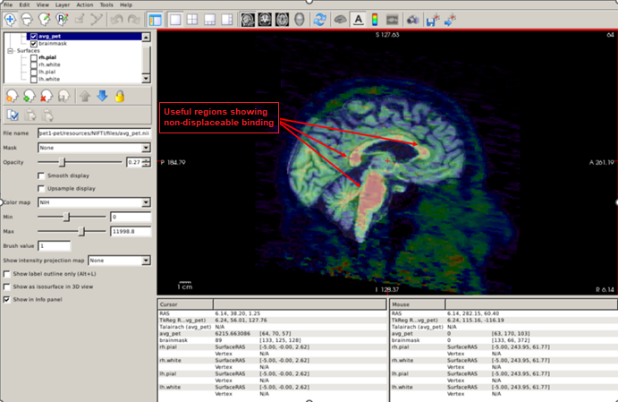
Amyloid PET images show non-displaceable binding (binding to something that is not amyloid plaques) in the white matter and brainstem. We can use this fact to check for correct coregistration. A useful strategy is to set the sagittal plane and visualize the brainstem and the corpus callosum, changing the opacity of the PET image to check that these regions with elevated signal do overlap:

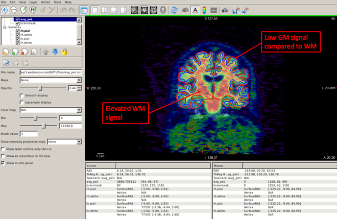
Another useful quality-control analysis is to set the pial and white surfaces in the coronal plane and check that the signal is elevated within the white matter boundary. Also, note the low uptake in the grey matter compared to the white matter, which suggests that this is an amyloid-negative individual.

Now that we checked that the coregistration is ok, we can run the commands to actually quantify our static PET scan. You can find these in the Stretch Your Knowledge section.

Stretch your knowledge

Visualizing cortical thickness maps

Labels are not the only thing we can overlay on the cortical surface. A very useful way to detect cortical atrophy with a single snapshot is to visualize cortical thickness maps of the brain. FreeSurfer provides regional, high spatial resolution measures of cortical thickness throughout the brain, allowing us to quantify regional atrophy across the brain when we don’t have any pre-specified hypothesis about the regions involved.

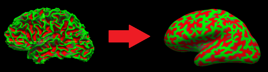
For better visualization of cortical thickness maps, particularly in the cortical sulci, we will use a surface known as the inflated surface. This surface essentially removes the folds by performing an inflation (similar to blowing up a beach ball) on the white surface, so that visualization on the sulci is easier:

Let’s see this in our CN subject. Let’s load both the white and inflated surfaces. Type:

freeview -f $SUBJECTS_DIR/CN/surf/lh.inflated $SUBJECTS_DIR/CN/surf/lh.white $SUBJECTS_DIR/CN/surf/rh.inflated $SUBJECTS_DIR/CN/surf/rh.white --viewport 3d

As you probably have guessed, lh(rh).inflated is the left (right) inflated surface. By default, Freeview represents sulci as red regions (based on a geometric property known as curvature) and gyri as green regions.

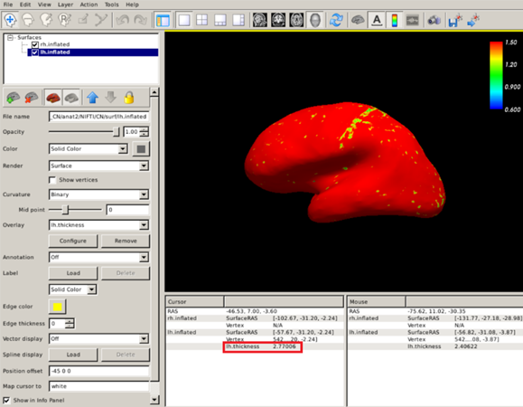
Now let’s visualize the cortical thickness map of our CN participant using the overlay option. Type:

freeview -f $SUBJECTS_DIR/CN/surf/lh.inflated:overlay=$SUBJECTS_DIR/CN/surf/lh.thickness:overlay_color=colorwheel,inverse:overlay_threshold=0.6,1.5 $SUBJECTS_DIR/CN/surf/rh.inflated:overlay=$SUBJECTS_DIR/CN/surf/rh.thickness:overlay_color=colorwheel,inverse:overlay_threshold=0.6,1.5 -colorscale --viewport 3d

Let’s break down this command a bit more:

As mentioned earlier, the -f option indicates which surface we want, in this case the left and right inflated surfaces.
We can specify multiple options to each surface by starting each one with a :. As you can see, this starts right after we have listed the name.
We use the overlay option to point to the left (right) cortical thickness map lh(rh).thickness.
We tell Freeview how to map colors to ranges of thickness values with the overlay_color option; here, we selected the inverted colorwheel scale (colorwheel, inverse).
Finally, we select the upper and lower limits of thickness values that this color map will represent with the overlay_threshold option; we select 0.6 mm as the lower and 1.5 mm as the maximum limit. All values below the minimum will use the minimum color and all thickness values greater than this maximum threshold will just have the maximum color. The colorscale flag will display the colorbar used.

If you want to measure cortical thickness in a particular region (vertex) you just have to click on the region you are interested in and check the number in the red box below (2.77 mm):

Exercise 4

Repeat the previous steps to visualize the cortical thickness maps of the AD and FTD patients with that of the CN subject. Use the inverted colorwheel as the colorscale and set colorscale lower and upper limits to 0.6 mm and 1.5 mm, respectively. Can you see clear differences among these subjects? What can the atrophy pattern tell us about the FTD patient?

Extracting quantitative PET metrics

To perform PET quantification, FreeSurfer requires the generation of a high-resolution segmentation called gtmseg.mgz. gtmseg.mgz will use aseg.mgz for subcortical structures, ?h.aparc.annot for cortical structures, and will estimate some extra-cerebral structures. To create gtmseg.mgz, we’d just need to run the following command (DON’T RUN THIS COMMAND, gtmseg TAKES 1-2 HOURS. WE’VE RUN gtmseg ALREADY FOR YOU):

gtmseg --s CN

This will create a file called $SUBJECTS_DIR/CN/mri/gtmseg.mgz, which is the anatomical 3D segmentation we are going to use to quantify our PET scan.

Now we just need to use the function mri_gtmpvc to get a table with the average signal values for each region of interest contained in gtmseg.mgz. Type:

mri_gtmpvc --i ~/oasis/OAS30015_PIB_d2144/static_PET.nii.gz --reg   ~/data/structural_mri_output/pet.reg.lta --seg   $SUBJECTS_DIR/CN/mri/gtmseg.mgz --auto-mask 1.01 --no-tfe --no-rescale --o ~/data/structural_mri_output/gtmpvc.output

As usual, the --i flag points to our static PET image we want to quantify.
The --reg points to the path of the registration file we obtained in the coregistration process.
The --seg flag points to the newly generated, high-resolution segmentation gtmseg.mgz.
The --auto-mask flag is to create a mask so that irrelevant voxels outside of the head are not analyzed (this is necessary only if we apply partial volume correction, but we need to specify it anyway); “1.01” will roughly extend the mask about 1mm beyond the head.
The --no-tfe flag disables the tissue fraction effect correction, which is a type of partial volume effect.
The --no-rescale flag indicates that we will get the raw PET values, without any rescaling.
Finally, the --o flag specifies the path in which the output of this quantification pipeline will be stored.

After running this, you will get an easy-to-read file called gtm.stats.dat containing the results of the quantification. The data has the following structure (here I used MATLAB and the function “readtable”)

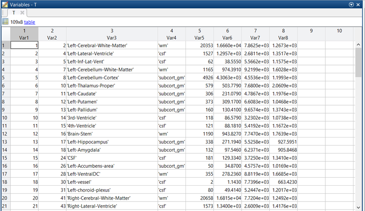
Var 1 (first column) is irrelevant. It is just the number of the row.
Var2 is the index of the ROI in the gtmseg.mgz segmentation.
Var 3 is the name of the ROI.
Var 4 is the tissue class (grey matter, white matter, csf, etc.)
Var 5 is the number of PET voxels in the ROI. This is important for computing weighted averages.
Var 6 and Var 8 are variance estimates that are not particularly interesting for us.
Var 7 is the actual PET signal, this is the quantity we are interested in.