A Practical Introduction to Working with Medical Image Data

Last updated on 2024-09-10 | Edit this page

Overview

Questions

How can we visualize volumetric data?
How do locations in an image get mapped to real-world coordinates?
How can we register different types of images together using ITK-SNAP?

Objectives

Describe the structure of medical imaging data and popular formats (DICOM and NifTi)
Discover and display medical imaging data in ITK-SNAP
Demonstrate how to convert between different medical image formats
Inspecting the NifTi header with nibabel
Manipulate image data (cropping images) with nibabel and learn how it is displayed on screen with ITK-SNAP

Medical Imaging Data

The Cancer Imaging Archive (TCIA)

In these exercises we will be working with real-world medical imaging data from the Cancer Imaging Archive (TCIA). TCIA is a resource of public datasets hosts a large archive of medical images of cancer accessible for public download.
We are using CT Ventilation as a Functional Imaging Modality for Lung Cancer Radiotherapy (also known as CT-vs-PET-Ventilation-Imaging dataset) from TCIA. The CT-vs-PET-Ventilation-Imaging collection is distributed under the Creative Commons Attribution 4.0 International License (https://creativecommons.org/licenses/by/4.0/). The CT-vs-PET-Ventilation-Imaging dataset contains 20 lung cancer patients underwent exhale/inhale breath hold CT (BHCT), free-breathing four-dimensional CT (4DCT) and Galligas PET ventilation scans in a single session on a combined 4DPET/CT scanner.

We recommend using the BHCT scans for participants CT-PET-VI-02 and CT-PET-VI-03 showing very little motion between inhale and exhale (for PET scan and accompanying CT scan), and BHCT scans for participants CT-PET-VI-05 and CT-PET-VI-07 (the inhale and exhale CT scans), where 05 has a different number of slices between the inhale and exhale.

Data paths contain: (A) inhale_BH_CT and exhale_BH_CT contain CT scans acquired during an inhalation breath hold and exhalation breath hold respectively, (B) PET contains a PET scan that measures the local lung function, and (C) CT_for_PET contains a CT scan acquired at the same time as the PET scan for attenuation correction of the PET scan and to provide anatomical reference for the PET data.

CT-PET-VI-02

BASH

├── CT-PET-VI-02
│   ├── CT_for_PET
│   ├── exhale_BH_CT
│   ├── inhale_BH_CT
│   └── PET

CT-PET-VI-03

BASH

/CT-PET-VI-03$ tree -d
├── CT-PET-VI-03
│   ├── CT_for_PET
│   └── PET

CT-PET-VI-05

BASH

CT-PET-VI-05$ tree -d
.
├── CT-PET-VI-05
│   ├── CT_for_PET
│   ├── exhale_BH_CT
│   ├── inhale_BH_CT
│   └── PET

CT-PET-VI-07

BASH

/CT-PET-VI-07$ tree -d
.
└── CT-PET-VI-07
    ├── exhale_BH_CT
    ├── inhale_BH_CT
    └── PET

For example, datasets in ITK-SNAP are illustrated in the following figures. Figure. CT-PET-VI-02 dataset

Refer to Summary and Setup section for further details on CT-vs-PET-Ventilation-Imaging dataset.

Data sharing ethics and policies

Data may require extensive cleaning and pre-processing before it is suitable to be used.
When using open datasets that contain images of humans, such as those from TCIA, for your own research, you will still need to get ethical approval as you do for any non-open datasets you use). This can usually be obtained from the local ethics committee (both Medical Physics and Computer Science have their own local ethics committee) or from UCL central ethics if your department does not have one.
Although there are many formats that medical imaging data can come in, we are going to focus on DICOM and NifTi as they are two of the most common formats. Most data that comes from a hospital will be in DICOM format, whereas NifTi is a very popular format in the medical image analysis community.

DICOM format

Digital Imaging and Communications in Medicine (DICOM) is a technical standard for the digital storage and transmission of medical images and related information. While DICOM images typically have a separate file for every slice, more modern DICOM images can come with all slices in a single file.

If you look at the data CT-PET-VI-02/CT_for_PET you will see there are 175 individual files corresponding to 175 slices in the volume. In addition to the image data for each slice, each file contains a header which can contain an extensive amount of extra information relating to the scan and subject.

In a clinical setting this will include patient identifiable information such as their name, address, and other relevant details. Such information should be removed before the data is transferred from the clinical network for use in research. If you ever discover patient identifiable information in the header of data you are using you should immediately alert your supervisor, manager or collaborator

The majority of the information in the DICOM header is not directly useful for typical image processing and analysis tasks. Furthermore, there are complicated ‘links’ (provided by unique identifiers, UIDs) between the DICOM headers of different files belonging to the same scan or subject. Together with DICOM routinely storing each slice as a separate files, it makes processing an entire imaging volume stored as DICOM format rather cumbersome, and the extra housekeeping required could lead to a greater chance of an error being made. Therefore, a common first step of any image processing pipeline is to convert the DICOM image to a more suitable format such as NifTi. Generally, most conversions go from DICOM to NIfTI. There are scenarios when you might want to convert from NIfTI back to DICOM, for example, if you need to import them into a clinical system that only works with DICOM.

Warning on converting images back to DICOM

Converting images back to DICOM such that they are correctly interpreted by a clinical system can be very tricky and requires a good understanding of the DICOM standard. More information on the DICOM standard can be found here: https://www.dicomstandard.org

NifTi format

The Neuroimaging Informatics Technology Initiative (NIfTI) image format are usually stored as a single file containing the imaging data and header information. While the NifTI file format was originally developed by the neuroimaging community it is not specific to neuroimaging and is now widely used for many different medical imaging applications outside of the brain. During these exercises you will learn about some of the key information stored in the NifTi header.

NifTI files can also store the header and image data in separate files but this is not very common. For more information, please see Anderson Winkler’s blog on the NIfTI-1 andNIfTI-2 formats.

Visualisation of volumetric data with ITK-SNAP

Getting Started with ITK-SNAP

Introduction

ITK-SNAP started in 1999 with SNAP (SNake Automatic Partitioning) and developed by Paul Yushkevich with the guidance of Guido Gerig. ITK-SNAP is open-source software distributed under the GNU General Public License. ITK-SNAP is written in C++ and it leverages the Insight Segmentation and Registration Toolkit (ITK) library. See Summary and Setup section for requirements and installation of ITK-SNAP

ITK-SNAP application

ITK-SNAP application shows three orthogonal slices and a fourth window for three-dimensional view segmentation.

Figure. Description of ITK-SNAP tools in the main window using MRI-crop example datasets for plane and 3D views.

Viewing and understanding DICOM data

We are using CT Lung DICOM dataset from CT-PET-VI-02/CT_for_PET, containing 175 dicom items and totalling 92.4 MB.

Opening and Viewing DICOM images

Open ITK-SNAP application
Load inhale scan using file browser
- Open the itk-snap application. If you have used it before it will display recent images when you open it, and you can select one of these to open it.
If the image you want to open is not listed under recent images, you can open it either by clicking the ‘Open Image…’ button at the bottom right of the window, or File->Open Main Image. When you do this a small window opens where you can enter the path of the file you want to open, or click Browse in your file explorer (exFinder in Mac and nautilus in Ubuntu) to open a file browser (for instance, “CT-PET-VI-02/CT_for_PET”). Do this and select the first slice from the Inhale_BH_CT folder, which is called 1-001.dcm. The set the File Format to DICOM Image Series and then click Next. You will then be asked to Select DICOM series to open, but as this folder only includes one series you can just click Next. Click Finish

Navigating DICOM images

Navigate around image, see intensity value, and adjust intensity window
To navigate around the image, i.e. change the displayed slices, you can left clicking in the displayed slices, using the mouse wheel, or the slider next to the displayed slices.
To zoom, you can use the right mouse button (or control + button 1), and pan using the centre mouse button (or alt + button 1).

Handling multiple DICOM images

We provide instructions for handling multiple DICOM images, applying overlays, viewing image information, and using color maps in ITK-SNAP. For this exmaple, we are using CT-PET-VI-02/inhale_BH_CT and CT-PET-VI-02/exhale_BH_CT dicoms.

Load additional image using `exhale_BH_CT` scan by drag and drop

Images can also be opened by simply dragging them on to the ITK-SNAP window. In a file explorer (Finder in Mac) go to the exhale_BH_CT folder and drag any of the dicom files on to the itksnap window. A small window will pop up asking What should itksnap do with this image? If you select Load as Main Image it will replace the current image. Instead select Load as Additional Image - this will enable easy comparison of the two images.

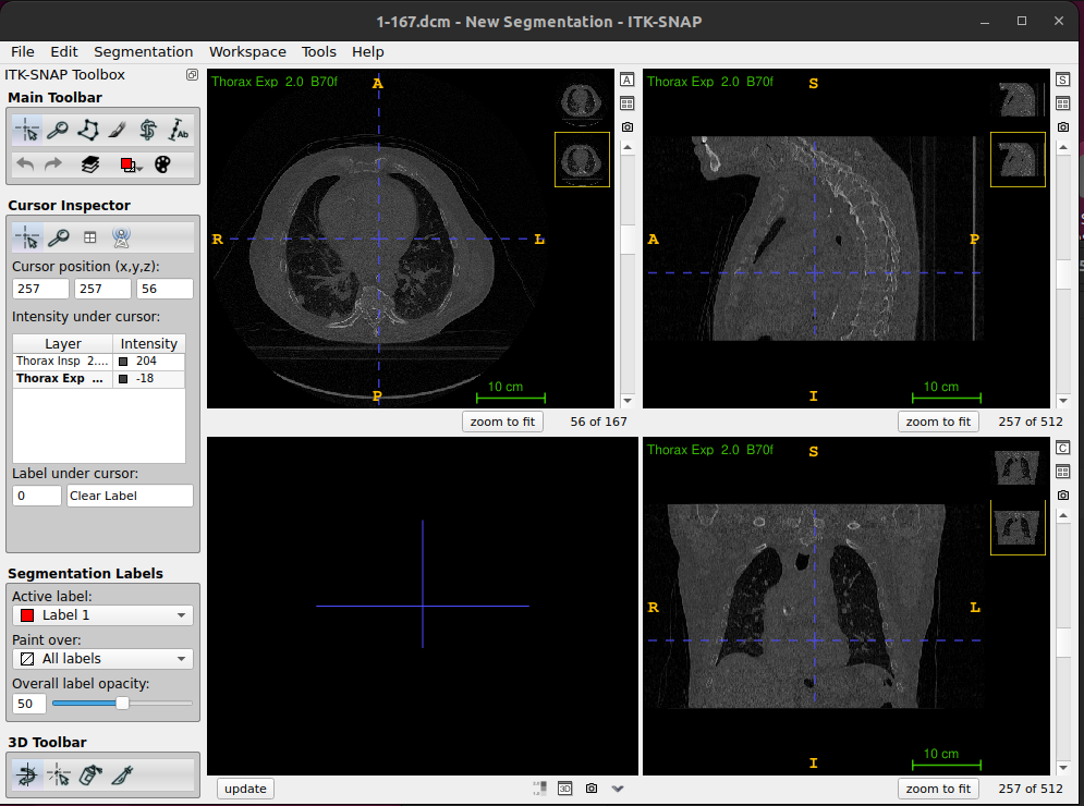
Using thumbnails to see image differences

Once the second image is loaded you will see two thumbnails in the top corner of each slice display
Click on these to swap the displayed slices from one image to the other - this will enable you to easily see the similarities and differences between the images.
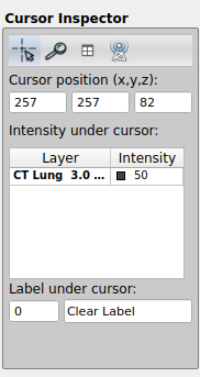
You will also see that both images now appear in the Cursor Inspector, where you can see the intensity value at the cursor for both images.
You can also change the displayed image by clicking on it in the Cursor Inspector

Figure. ITK-SNAP thumbnails, handlding two DICOM images (inhale_BH_CT and exhale_BH_CT for CT-PET-VI-02)

Colour overlay

In some cases you may want to display an image as a colour overlay on top of another image, e.g. displaying a PET image overlaid on the corresponding CT.

Colour overlay as a separate image (shown besides other images)

Load Primary Image:
- Open your primary DICOM series of the CT-PET-VI-02/CT_for_PET image either using the drag and drop method or File->Open Image as described above.
- Make sure File Format is DICOM Image Series.
- This time select Load as Main Image. This will load in the new image replacing the two that were previously loaded.
Load Overlay Image:
- Load the CT-PET-VI-02/PET image either using the drag and drop method or File->Open Image

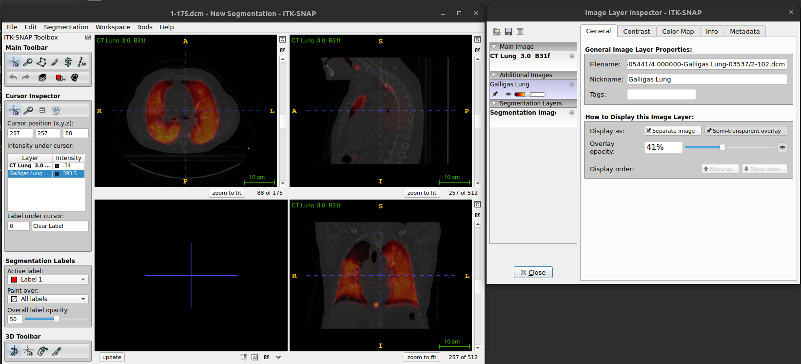
Colour overlay as a semi-transparent overlay (shown on the top of other images)

Load Primary Image:
- Open your primary DICOM series of the CT-PET-VI-02/CT_for_PET image either using the drag and drop method or File->Open Image as described above.
- Make sure File Format is DICOM Image Series.
- Select Load as Main Image.
Load Overlay Image:
- Load the CT-PET-VI-02/PET image either using the drag and drop method or File->Open Image
- When the image has loaded select As a semi-transparent overlay. You can also set the overlay color map here - select Hot from the drop-down menu and click Next.
- The image summary will then be displayed, along with a warning about possible loss of precision (which can be ignored). Click Finish

Figure. ITK-SNAP semi-transparent overlays

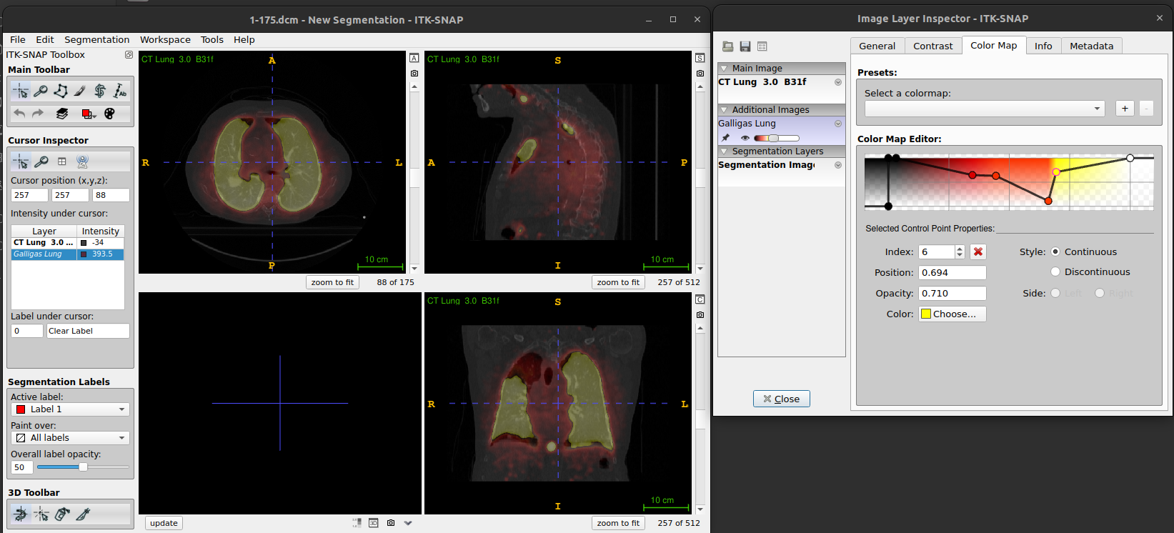
Layer inspector tools

Load CT-PET-VI-02/CT_for_PET and CT-PET-VI-02/PET scan datasets, using hot semi-transparency (as shown above).
Go to Tools->Layer Inspector. This opens the Image Layer Inspector window. You will see the two images on the left, and five tabs along the top of the window.
PET image appears in Cursor Inspector (called Galligas Lung) in italic and CT image as CT Lung in bold.
The General tab displays the filename and the nickname for the selected image.
- The Nickname can be edited. For the PET image the general tab also displays a slider to set the opacity, and the option to display it as a separate image or semi-transparent overlay.

Figure. ITK-SNAP: Layer inspector with general tab

The Contrast tab enables you to adjust how the image intensities are displayed for the different images, e.g. Select the lung image and set the maximum value to 1000 (push enter after typing the number) and this will make the structures in the lung easier to see.

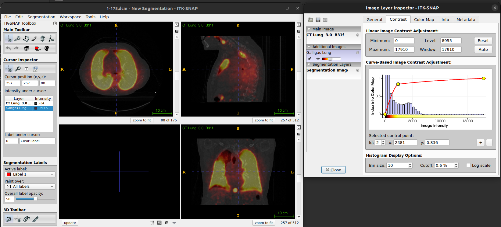
Figure. ITK-SNAP: Layer inspector with contrast tab

The color map tab can be used to select and manipulate the colour map
- One of the key elements of an imaging viewer is to provide different means to map those values into grey scales or different colors.
- We will show you how to apply different color maps or lookup tables to your data and how this affects how the images are presented to the user.
1. Load the Image: - Open the desired DICOM series.
2. Open Color Map Settings: - Go to Tools > Color Maps Editor.
3. Apply and Adjust Color Map: - Choose a predefined color map from the list. You might also create a customised map. - Adjust the intensity and transparency settings as needed to enhance the visualisation of the images.

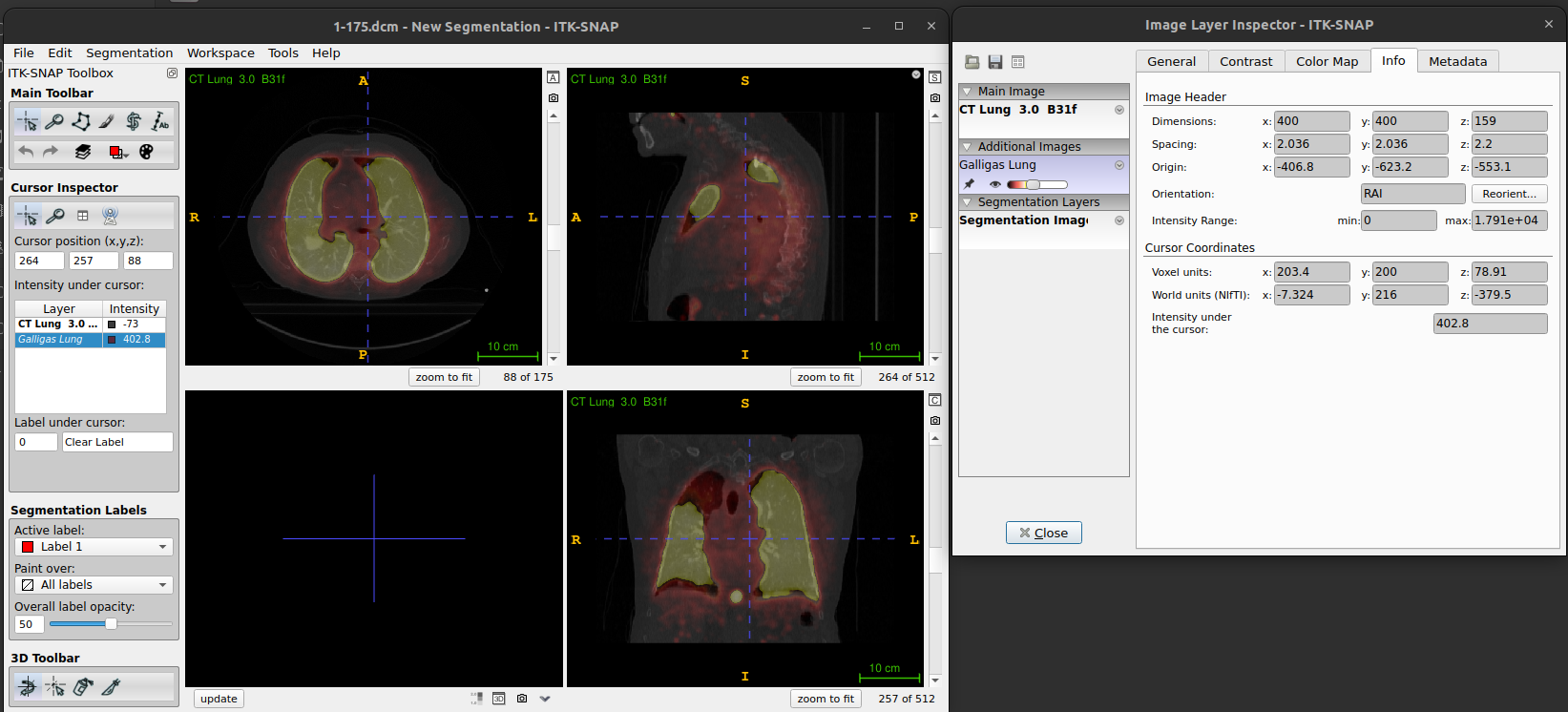
Figure. ITK-SNAP: Layer inspector with color map tab

The info tab displays the Image Header information for the images and also gives the Cursor Coordinates in both Voxel and World units.
- A dialog box will appear displaying metadata and other relevant information about the loaded DICOM images (e.g. values for image header and cursor coordinates).
- If you look at the info tab for both the CT image and PET image you will see that the header information for the images is different, and the cursor coordinates in voxel units for the PET image are not whole numbers.
- This is because the displayed slices are from the main (CT) image, and the overlaid (PET) image slices are interpolated at the corresponding locations.

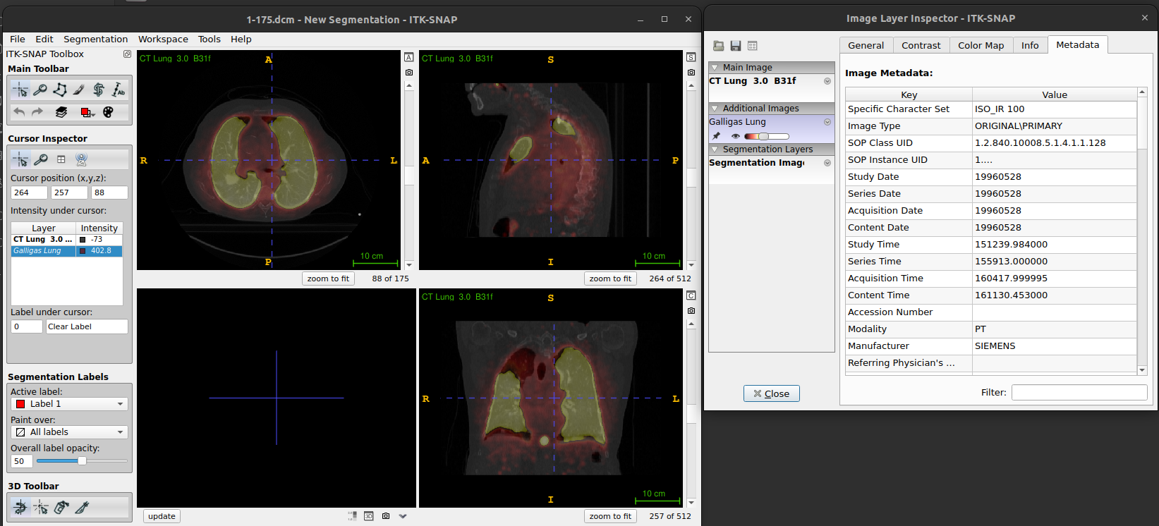
Figure. ITK-SNAP: Layer inspector with info tab

The metadata tab contains (some of) the information from the DICOM header of the images

Figure. ITK-SNAP: Layer inspector with metadata tab

Converting DICOM images to NifTi

As mentioned earlier in the exercise, the NIfTI image format tends to be much easier to work with when processing and analysing medical image data. We will now work on converting DICOM images to a NIfTI image volume.

Using ITK-SNAP

In the ITK-SNAP application, save the file by clicking ‘File’ –> ‘Save image’ –> rename image and choose format as ‘NiFTI’.

Warning for Linux users.

You might get this error Error: exception occurred during image IO. Exception: std::expedition to which we suggest using dicom2nifti library.

Using dicom2nifti

Open terminal, activate mirVE environment and run python

BASH

conda activate mirVE
python

Run the following commands to convert your DICOM scans to nifti format.

PYTHON

from pathlib import Path 
import dicom2nifti 
dicom_path = Path("CT_for_PET")
dicom2nifti.convert_directory(dicom_path, ".", compression=True, reorient=True)
pet_dicom_path = Path("PET")
dicom2nifti.convert_directory(pet_dicom_path, ".", compression=True, reorient=True)

Creating the following files:

`3_ct_lung__30__b31f.nii.gz` [47M] and renamed as `ct_for_pet.nii.gz`
`4_galligas_lung.nii.gz` [12M] and renamed as `pet.nii.gz`

Using others packages

You might also be interested to look other packages: * https://github.com/rordenlab/dcm2niix * https://nipy.org/nibabel/dicom/dicom.html#dicom * https://neuroimaging-cookbook.github.io/recipes/dcm2nii_recipe/

Viewing and understanding the NifTi header with NiBabel

We are going to use the python package NiBabel to upload NifTI images and learn some basic properties of the image using Nibabel. nibabel api provides various image utilities, conversions methods, helpers. We recommend to checking documentation for further deatils on using nibabel library. Please see instructions to install NiBabel package and other dependecies.

Loading images

Open terminal, activate mirVE environment and run python

BASH

conda activate mirVE
python

Importing python packages under */episodes path

A NifTi image with extension *.nii.gz can be read using nibabel’s load function.

PYTHON

import numpy as np
import nibabel as nib
import matplotlib.pyplot as plt
nii3ct = nib.load("data/ct_for_pet.nii.gz")

`NiBabel`'s `load` function does not actually read the image data itself from disk, but
does read and interpret the header, and provides functions for accessing the image data.
Calling these functions reads the data from disk (unless it has already been read, in which
case it may be cached in memory already.

NifTI object type, shape/size The Nifti1Image object allows us to see the size/shape of the image and its data type.

PYTHON

print(type(nii3ct))
# <class 'nibabel.nifti1.Nifti1Image'>

PYTHON

print(nii3ct.get_data_dtype())
#int16

PYTHON

nii3ct.shape
# (512, 512, 175)

Affine transform, mapping from voxel space to world space There are two common ways of specifying the affine transformation mapping from voxel coordinates to world coordinates in the nifti header, called the sform and the `qform’. Another transformation is that neither the sform or qform is used the mapping is performed based just on the voxel dimensions. The sform directly stores the affine transformation in the header whereas the qform stores the affine transformation using quaternions.

Recommending sform over qform

We strongly advise always using the sform over the qform, as: * It is easier to understand (at least for instructors). * It can contain shears which cannot be represented using the qform.

PYTHON

nii3ct.affine
#array([[  -0.9765625 ,    0.        ,    0.        ,  249.51171875],
#       [  -0.        ,    0.9765625 ,    0.        ,  -33.01171875],
#       [   0.        ,   -0.        ,    2.        , -553.5       ],
#       [   0.        ,    0.        ,    0.        ,    1.        ]])

Header features

Printing nii3ct.header outputs

PYTHON

print(nii3ct.header)

#<class 'nibabel.nifti1.Nifti1Header'> object, endian='<'
#sizeof_hdr      : 348
#data_type       : b''
#db_name         : b''
#extents         : 0
#session_error   : 0
#regular         : b''
#dim_info        : 0
#dim             : [  3 512 512 175   1   1   1   1]
#intent_p1       : 0.0
#intent_p2       : 0.0
#intent_p3       : 0.0
#intent_code     : none
#datatype        : int16
#bitpix          : 16
#slice_start     : 0
#pixdim          : [-1.         0.9765625  0.9765625  2.         1.         1.
#  1.         1.       ]
#vox_offset      : 0.0
#scl_slope       : nan
#scl_inter       : nan
#slice_end       : 0
#slice_code      : unknown
#xyzt_units      : 2
#cal_max         : 0.0
#cal_min         : 0.0
#slice_duration  : 0.0
#toffset         : 0.0
#glmax           : 0
#glmin           : 0
#descrip         : b''
#aux_file        : b''
#qform_code      : unknown
#sform_code      : aligned
#quatern_b       : 0.0
#quatern_c       : 1.0
#quatern_d       : 0.0
#qoffset_x       : 249.51172
#qoffset_y       : -33.01172
#qoffset_z       : -553.5
#srow_x          : [ -0.9765625   0.          0.        249.51172  ]
#srow_y          : [ -0.          0.9765625   0.        -33.01172  ]
#srow_z          : [   0.    -0.     2.  -553.5]
#intent_name     : b''
#magic           : b'n+1'

sform transformation matrix You can see that the sform is stored in the srow_x, srow_y, and srow_z fields of the header. These specify the top three rows of a 4x4 matrix representing an affine transformation using homogeneous coordinates. The fourth row is not stored as it is always [0 0 0 1]. You will notice that the sform matrix matches the affine transform in the Nifti1Image object.
sform_code and qform_code It can also be seen from the sform_code and qform_code that both the sform and qform are set for this image. There are 5 different sform/qform codes defined:

Code	Label	Meaning
0	unknown	sform not defined
1	scanner	RAS+ is scanner coordinates
2	aligned	RAS+ aligned to some other scan
3	talairach	RAS+ in Talairach atlas space
4	mni	RAS+ in MNI atlas space

Which code to use?

But for most purposes all that matters is whether the code is unknown (numerical value 0) or one of the other valid values. If the code is unknown then the sform/qform is not specified (and any values provided in the sform/qform fields of the header will be ignored). For any other valid values the sform/qform is specified and the affine transform will be determined from the corresponding header values.

`qform` transform

You can also see qform transform using the get_qform function, which returns the affine matrix represented by the qform:

PYTHON

print(nii3ct.get_qform())
#[[  -0.9765625     0.            0.          249.51171875]
# [   0.            0.9765625     0.          -33.01171875]
# [   0.            0.            2.         -553.5       ]
# [   0.            0.            0.            1.        ]]

Advincing on using sform

However, the nifti format does not require that the sform and qform specify the same matrix. It is also not well defined what should be done when they are both provided and are different from each other. Often the qform is simply ignored and the sform is used, so the general advice is to only use the sform and set the qform to unknown to avoid any confusion.

Coordinate system

LPS

The original DICOM images assume the world coordinate system is LPS (i.e. values increase when moving to the left, posterior, and superior). See this helpful information on DICOM orientations, and determine if you obtained a similar affine transform from the DICOM headers. The values in the first two rows corresponding to the x and y dimensions would be the negative of those in the NifTi header.

RAS

You will notice that the diagonal elements of the affine matrix match the voxel dimensions (as the affine matrix does not contain any rotations), but the values for the x and y dimensions are negative. This is because the voxel indices increase as you move to the left and posterior of the image/patient, but the nifti format assumes a RAS world coordinate system (i.e. the values increase as you move to the right and anterior of the patient). Therefore, the world coordinates decrease as the voxel indices increase.

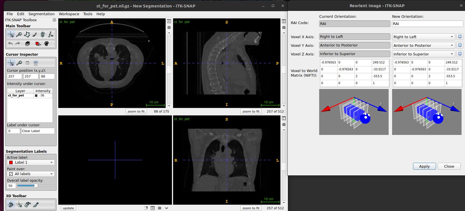
ITK-SNAP visualisation coordinate system

ITK-SNAP provides the option, Tools>Reorient Image, to set image orientation using three-letter code (RAI code), describing the image rows, columns, and slice map to the anatomical coordinates. For example, the code ASL means that image rows (X) run from Anterior to Posterior, image columns (Y) run from Superior to Inferior, and images slices (Z) run from Left to Right.

Modifying `NifTi` images and headers with Nibabel

Obtaining image pixel data

The image data for a Nifti1Image object can be accessed using the get_fdata function. This will load the data from disk and cast it to float64 type before returning the data as a numpy array.

PYTHON

image_data=nii3ct.get_fdata()
print(type(image_data))
#<class 'numpy.ndarray'>

print(image_data.dtype, image_data.shape)
#float64 (512, 512, 175)

You can also plot a particular slide, (e.g. 140) for such data.

PYTHON

plt.imshow(image_data[:,:,140], cmap="gray"); plt.show()
#launch plot window

Using float64 data type

Casting image data to float64 prevents any integer-related errors and problems in downstream processing when using the data read by NiBabel. However, this does not change the type of the image stored on disk, which as we have seen is int16 for this image, and this could still lead to downstream errors or unexpected behaviour for any processing that works directly on the images stored on disk. We are going to convert the image saved on disk to a floating point image, using the set_data_dtype function to set the data type to float32. Essentially, we are going to use 32 bit rather than 64 bit floating point, as this is usually sufficiently accurate.

PYTHON

print(nii3ct.get_data_dtype())
#int16

PYTHON

nii3ct.set_data_dtype(np.float32)
print(nii3ct.get_data_dtype())
#float32

We are also going to set the qform to unknown, updating the corresponding fields in the header. We use the set_qform function to set the qform code. To just set the code and not modify the other qform values in the header, the first input should be None. It is not necessary to modify the other qform values as they should be ignored when the code is set to unknown.

PYTHON

nii3ct.set_qform(None, code = 'unknown')
print(nii3ct.header)
...
qform_code      : unknown
...

The floating point image can now be written to disk using the save function.

We do not need to manually modify the type of the image data?

Setting the data type for the Nifti1Image object tells it which type to use when writing the image data to disk.

PYTHON

nib.save(nii3ct, 'data/ct_for_pet_float32.nii.gz')

16-bit integers vs 32 bit floats

The file size of ct_for_pet_float32.nii.gz is larger than ct_for_pet.nii.gz (61 MB, 47 MB, respectively) because of the conversion from 16 bit integers to 32 bit floats. Both images are compressed, but the compression is more efficient for the floating point image: while a 32-bit floating point variable is twice the size of a 16-bit integer, the floating image is less than double the size of the original integer image.

int16

PYTHON

nii3ct_int16 = nib.load("data/ct_for_pet.nii.gz")

PYTHON

print(nii3ct_int16.get_data_dtype())
#int16

PYTHON

print(nii3ct_int16.header)
#<class 'nibabel.nifti1.Nifti1Header'> object, endian='<'
#sizeof_hdr      : 348
#data_type       : b''
#db_name         : b''
#extents         : 0
#session_error   : 0
#regular         : b''
#dim_info        : 0
#dim             : [  3 512 512 175   1   1   1   1]
#intent_p1       : 0.0
#intent_p2       : 0.0
#intent_p3       : 0.0
#intent_code     : none
#datatype        : int16
#bitpix          : 16
#slice_start     : 0
#pixdim          : [-1.         0.9765625  0.9765625  2.         1.         1.
#  1.         1.       ]
#vox_offset      : 0.0
#scl_slope       : nan
#scl_inter       : nan
#slice_end       : 0
#slice_code      : unknown
#xyzt_units      : 2
#cal_max         : 0.0
#cal_min         : 0.0
#slice_duration  : 0.0
#toffset         : 0.0
#glmax           : 0
#glmin           : 0
#descrip         : b''
#aux_file        : b''
#qform_code      : unknown
#sform_code      : aligned
#quatern_b       : 0.0
#quatern_c       : 1.0
#quatern_d       : 0.0
#qoffset_x       : 249.51172
#qoffset_y       : -33.01172
#qoffset_z       : -553.5
#srow_x          : [ -0.9765625   0.          0.        249.51172  ]
#srow_y          : [ -0.          0.9765625   0.        -33.01172  ]
#srow_z          : [   0.    -0.     2.  -553.5]
#intent_name     : b''
#magic           : b'n+1'

float32

PYTHON

nii3ct_float32 = nib.load("data/ct_for_pet_float32.nii.gz")

PYTHON

print(nii3ct_float32.get_data_dtype())
#float32

PYTHON

print(nii3ct_float32.header)
#<class 'nibabel.nifti1.Nifti1Header'> object, endian='<'
#sizeof_hdr      : 348
#data_type       : b''
#db_name         : b''
#extents         : 0
#session_error   : 0
#regular         : b''
#dim_info        : 0
#dim             : [  3 512 512 175   1   1   1   1]
#intent_p1       : 0.0
#intent_p2       : 0.0
#intent_p3       : 0.0
#intent_code     : none
#datatype        : float32
#bitpix          : 32
#slice_start     : 0
#pixdim          : [-1.         0.9765625  0.9765625  2.         1.         1.
#  1.         1.       ]
#vox_offset      : 0.0
#scl_slope       : nan
#scl_inter       : nan
#slice_end       : 0
#slice_code      : unknown
#xyzt_units      : 2
#cal_max         : 0.0
#cal_min         : 0.0
#slice_duration  : 0.0
#toffset         : 0.0
#glmax           : 0
#glmin           : 0
#descrip         : b''
#aux_file        : b''
#qform_code      : unknown
#sform_code      : aligned
#quatern_b       : 0.0
#quatern_c       : 1.0
#quatern_d       : 0.0
#qoffset_x       : 249.51172
#qoffset_y       : -33.01172
#qoffset_z       : -553.5
#srow_x          : [ -0.9765625   0.          0.        249.51172  ]
#srow_y          : [ -0.          0.9765625   0.        -33.01172  ]
#srow_z          : [   0.    -0.     2.  -553.5]
#intent_name     : b''
#magic           : b'n+1'

ITK-SNAP visualistaion of 16-bit integers vs 32 bit floats

Figure. ITK-SNAP: Metadata for 16-bit integers vs 32-bit floats

Cropping data

Cropping data might often contain background voxels which can be useful in some instances but might take up valuable RAM memory, especially for large images. We are going to crop the image from slice 103 to slice 381 in the x dimension (Sagittal slices) and from slice 160 to 340 in the y dimension (Coronal slices). Use ITK-SNAP to confirm that cropping the image to these slices will only remove slices that do not contain the patient.

Notes on Nifti1Image object

It is not possible to change the image data in a Nifti1Image object, e.g. to use a smaller array corresponding to a cropped image. Therefore, if you want to modify the image data you need to create a new array with the modified data, then create a new Nifti1Image object using this new array which is used to save the modified image to disk.

Read the image data from disk using get_fdata and then create a new array containing a copy of the desired slices:

PYTHON

nii3ct_float32 = nib.load("data/ct_for_pet_float32.nii.gz")
nii3ct_float32.set_data_dtype(np.float32)
print(nii3ct_float32.get_data_dtype())
#float32

PYTHON

image_data=nii3ct_float32.get_fdata()
print(image_data.dtype, image_data.shape)
#float64 (512, 512, 175)

PYTHON

plt.imshow(image_data[:,:,100], cmap="gray"); plt.show()
#launch plot window

PYTHON

image_data_cropped = image_data[103:381,160:340,:].copy()
#x[sagittal], y[coronal], z[axial] #voxel units

Notes on copying data

It is important to create a copy of the data (using the copy function, as show above). Otherwise the new image will reference the data in the original image, and if you make any changes to the values in the new image they will also be changed in the original image.

When creating a new Nifti1Image object you can provide an affine transform and/or a Nifti1Header object (e.g. nii_1.header). When you just provide an affine, a default header is created with the sform set according to the provided affine transform and the qform set to unknown. When you provide a header, the values in it will be copied into the header for the new image, except that the dim values will be updated based on the image data provided. If you provide an affine as well as a header, and the affine is different to the sform or qform in the header they will be set to the provided affine and unknown respectively. If the affine is not provided, it is not set from the header but left empty. So, if any of your downstream processing will make use of the affine, make sure you manually set it from the header either when creating the Nifti1Image object or by calling the set_sform or set_qform functions for the object (which update the affine as well as setting the sform/qform). Here we will provide a Nifti1Header object as we want the header for the new image to based on the uncropped image and will use the sform from the header as the affine for the new Nifti1Image.

PYTHON

nii3ct_float32_cropped = nib.nifti1.Nifti1Image(image_data_cropped, nii3ct_float32.get_sform(), nii3ct_float32.header)
nii3ct_float32_cropped.shape
#(278, 180, 175)

PYTHON

print(nii3ct_float32_cropped.header)
#<class 'nibabel.nifti1.Nifti1Header'> object, endian='<'
#sizeof_hdr      : 348
#data_type       : b''
#db_name         : b''
#extents         : 0
#session_error   : 0
#regular         : b''
#dim_info        : 0
#dim             : [  3 278 180 175   1   1   1   1]
#intent_p1       : 0.0
#intent_p2       : 0.0
#intent_p3       : 0.0
#intent_code     : none
#datatype        : float32
#bitpix          : 32
#slice_start     : 0
#pixdim          : [-1.         0.9765625  0.9765625  2.         1.         1.
#  1.         1.       ]
#vox_offset      : 0.0
#scl_slope       : nan
#scl_inter       : nan
#slice_end       : 0
#slice_code      : unknown
#xyzt_units      : 2
#cal_max         : 0.0
#cal_min         : 0.0
#slice_duration  : 0.0
#toffset         : 0.0
#glmax           : 0
#glmin           : 0
#descrip         : b''
#aux_file        : b''
#qform_code      : unknown
#sform_code      : aligned
#quatern_b       : 0.0
#quatern_c       : 1.0
#quatern_d       : 0.0
#qoffset_x       : 249.51172
#qoffset_y       : -33.01172
#qoffset_z       : -553.5
#srow_x          : [ -0.9765625   0.          0.        249.51172  ]
#srow_y          : [ -0.          0.9765625   0.        -33.01172  ]
#srow_z          : [   0.    -0.     2.  -553.5]
#intent_name     : b''
#magic           : b'n+1'

The cropped image can now be saved using Nibabel’s save function.

PYTHON

nib.save(nii3ct_float32_cropped, "data/ct_for_pet_cropped.nii.gz")

Now load the cropped image into ITK-SNAP. You will see that the image has been cropped in the x and y dimensions as expected, but it is shifted relative to the uncropped image:

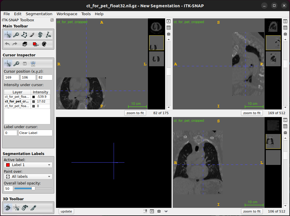
Figure. ITK-SNAP: Cropped image in ITK-SNAP

This is because we did not update the origin/offset in the nifti header to account for the slices we removed. The origin gives the world coordinates of the voxel (0, 0, 0). So, if we want the images to remain aligned, we need to set the origin for the cropped image to be the same as the world coordinates of voxel (103, 160, 0) in the uncropped image. This can be calculated using the affine from the uncropped image, and used to create a new affine matrix with this as the origin (the origin is the top 3 values in the 4th column of the matrix). The new affine matrix can then be used to set the sform (which also sets the affine) for the cropped image, which can then be saved.

PYTHON

cropped_origin = nii3ct_float32.affine@np.array([103,160,0,1])
cropped_origin
#array([ 148.92578125,  123.23828125, -553.5       ,    1.        ])

PYTHON

aff_mat_cropped = nii3ct_float32_cropped.get_sform()
print(aff_mat_cropped)
#[[  -0.9765625     0.            0.          249.51171875]
# [  -0.            0.9765625     0.          -33.01171875]
# [   0.           -0.            2.         -553.5       ]
# [   0.            0.            0.            1.        ]]

PYTHON

aff_mat_cropped[:, 3] = cropped_origin
print(aff_mat_cropped)
#[[  -0.9765625     0.            0.          148.92578125]
# [  -0.            0.9765625     0.          123.23828125]
# [   0.           -0.            2.         -553.5       ]
# [   0.            0.            0.            1.        ]]

Note, NiBabel provides handy functionality for slicing nifti images and updating the affine transforms and header accordingly using the slicer attribute:

PYTHON

nii3ct_float32_cropped.set_sform(aff_mat_cropped)
nii3ct_float32_cropped.affine
#array([[  -0.9765625 ,    0.        ,    0.        ,  148.92578125],
#       [  -0.        ,    0.9765625 ,    0.        ,  123.23828125],
#       [   0.        ,   -0.        ,    2.        , -553.5       ],
#       [   0.        ,    0.        ,    0.        ,    1.        ]])

PYTHON

nib.save(nii3ct_float32_cropped, "data/ct_for_pet_float32_cropped_affine.nii.gz")

updating the affine transforms with nibabel.slicer

PYTHON

nii3ct_float32_cropped_with_nibabel_slicer = nii3ct_float32.slicer[103:381,160:340,:]
nii3ct_float32_cropped_with_nibabel_slicer.affine
#array([[  -0.9765625 ,    0.        ,    0.        ,  148.92578125],
#       [   0.        ,    0.9765625 ,    0.        ,  123.23828125],
#       [   0.        ,    0.        ,    2.        , -553.5       ],
#       [   0.        ,    0.        ,    0.        ,    1.        ]])

But you wouldn’t have learnt so much if we’d simply done that to start with :)

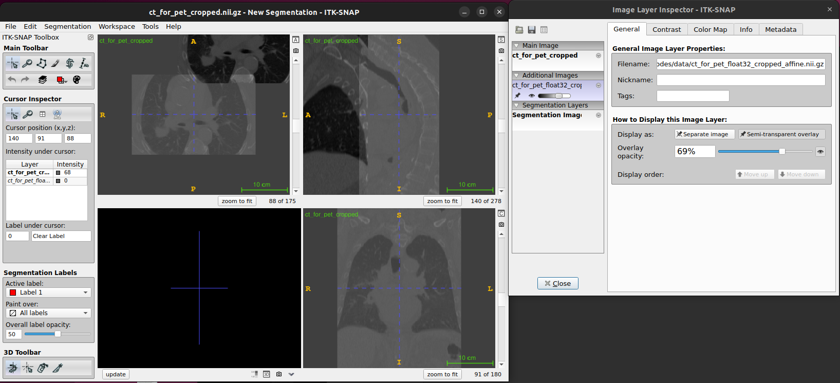
If you load the cropped and aligned image into ITK-SNAP using overlay semi-transparent feature, you will see that it is now aligned with the original image but has fewer slices in the x and y dimensions.

If we try to perform a registration between these images as they are, it will likely have difficulties as the images are so far out of alignment to start with. One way to roughly align the images prior to performing a registration is to align the centres of the images by modifying the origin for the 2nd subject such that the image centres for both images have the same world coordinates.

This can be done by following these steps:
* Load ct_for_pet_cropped.nii.gz
* Calculate the centre of this image in voxel coordinates
* Calculate the centre of this image in world coordinates
* Calculate the centre of the cropped image from subject 1 in voxel coordinates
* Calculate the centre of the cropped image from subject 1 in world coordinates
* Calculate the translation (in world coordinates) required to align the images: Centre image 1 = centre image 2 + translation

Add this translation to the origin for image 2 Save the image for image 2 using the header with the updated origin Try and write code to implement these steps yourself, based on what you have learnt so far. If you get stuck ask me or one of the PGTAs for help.

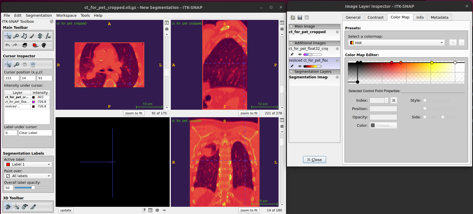
If you have implemented this correctly when you load the aligned image from image 2 into ITK-SNAP is should appear roughly aligned with the images from image 1. You can use Color Map feature tab and the scroll bar to see the differences between two images.

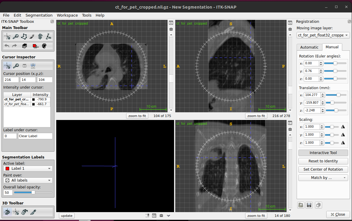
Cropped and aligned image

Automated image registrations can be prone to be failure if there are very large initial differences between the images. A manual alignment is subjective, but can provide a good enough starting guess that keeps the objective, automated registration more reliable.
* Manually aligning images For manual image registration in ITK-SNAP go to Tools > image registration

Automatic registration (affine)
You can use niftyreg, Reg_aladin or DL methods.

References

NiBabel: “The NiBabel documentation also contains some useful information and tutorials for working with NifTi images and understanding world coordinate systems and radiological vs neurological view.”
ITK-SNAP:
- Tutorial: Getting Started with ITK-SnAP
- ITK-SNAP 3.x Training Class Final Program
AI-based medical image registration:

A Practical Introduction to Working with Medical Image Data

Overview

Questions

Objectives

Medical Imaging Data

The Cancer Imaging Archive (TCIA)

BASH

BASH

BASH

BASH

Data sharing ethics and policies

DICOM format

Warning on converting images back to DICOM

NifTi format

Visualisation of volumetric data with ITK-SNAP

Getting Started with ITK-SNAP

Introduction

ITK-SNAP application

Viewing and understanding DICOM data

Opening and Viewing DICOM images

Navigating DICOM images

Handling multiple DICOM images

Load additional image using exhale_BH_CT scan by drag and drop

Using thumbnails to see image differences

Colour overlay

Colour overlay as a separate image (shown besides other images)

Colour overlay as a semi-transparent overlay (shown on the top of other images)

Layer inspector tools

Converting DICOM images to NifTi

Using ITK-SNAP

Warning for Linux users.

Using dicom2nifti

BASH

PYTHON

Using others packages

Viewing and understanding the NifTi header with NiBabel

Loading images

BASH

PYTHON

PYTHON

PYTHON

PYTHON

Recommending sform over qform

PYTHON

Header features

PYTHON

Which code to use?

qform transform

PYTHON

Advincing on using sform

Coordinate system

LPS

RAS

ITK-SNAP visualisation coordinate system

Modifying NifTi images and headers with Nibabel

Obtaining image pixel data

PYTHON

PYTHON

Using float64 data type

PYTHON

PYTHON

PYTHON

We do not need to manually modify the type of the image data?

PYTHON

16-bit integers vs 32 bit floats

PYTHON

PYTHON

PYTHON

PYTHON

PYTHON

PYTHON

ITK-SNAP visualistaion of 16-bit integers vs 32 bit floats

Cropping data

Notes on Nifti1Image object

PYTHON

PYTHON

PYTHON

PYTHON

Notes on copying data

PYTHON

Load additional image using `exhale_BH_CT` scan by drag and drop

`qform` transform

Modifying `NifTi` images and headers with Nibabel